0The puzzle
A Transformer’s attention lets every token look at every other token. Each look is a single comparison: the token that asks (the query) scores one other token (a key) at a time, and the layer takes a weighted average of what the high-scoring tokens carry. Researchers have also built layers that score pairs of tokens, or chains of tokens, and their record is strangely uneven.
In some places these higher-order layers are the heart of the system. AlphaFold, which predicts the shapes of proteins, keeps a state for every pair of amino acids and updates each pair through a third one1. The same pattern is the core of the Edge Transformer, a model of systematic compositional parsing2. Elsewhere it adds little: in language modelling, attention over pairs of tokens gives small gains in average loss3,4, with larger ones on mathematics, coding, reasoning and logic3.
Meanwhile, ordinary Transformers fail at tasks that look easy. Trained to find a path through a graph, they stop converging as the graphs grow5, although theory shows that attention can represent connectivity with only logarithmically many layers6. Trained on the card game SET, a Transformer memorises its training deals long before it learns the rule, and learns the rule only after seeing many distinct questions.
So there are two puzzles. Why do higher-order layers help so much in some places and so little in others? And why does a Transformer fail to learn tasks that it can, in principle, represent?
The paper’s answer is to look at what a layer adds up. Every attention-like layer computes, for each query, a weighted sum over some collection of objects: single tokens, pairs of tokens, routes through a graph, groups of tokens. The paper calls the objects that a task’s answer depends on its witnesses, and the collection a layer sums over its family. When the layer’s family matches the task’s witnesses, the layer learns easily. When it does not, each token must first build the missing structure into its own state, and that is where training fails. The title borrows a courtroom image: a verdict can be no better than the witnesses who are called.
Here is where the tutorial goes. Chapter 2 writes every layer in one form, a weighted sum over a family read out at a “temperature” that sets how sharply the best candidates win. From that form come three principles and two theorems: a depth law for how far stacked pair layers can see along a graph (Chapter 3) and a size law for how sharp a read-out must be as the number of candidates grows (Chapter 5). New layers built on them learn where Transformers fail:
- one layer that adds up every route through a graph at once, trained on graphs of 49 vertices, answers every question at every search depth on graphs of 250 vertices, in each of three runs (Chapter 3);
- a layer that adds up all pairs of cards in time proportional to the number of cards, when told that SET’s values wrap around after three, learns SET from as few examples as a pair-attention layer and, trained on tables of 8 cards, works on tables of 20 (Chapter 4);
- on twelve graph-algorithm tasks of a standard benchmark, one small block of 186,000 parameters, run repeatedly, matches (within half a percentage point) or beats a model of at least 73 million parameters on 9 of 12 tasks of the official test set, and on 8 of 12 with freshly drawn test graphs (Chapter 6).
The same account explains where pair layers did not help (language and chess, at the scales tested) and where a parallel layer must loop many times (Chapter 6). The positive results are on synthetic and algorithmic tasks, with small models; Chapter 7 states the limits.
1Prerequisites
This chapter teaches four things: attention as a soft lookup, softmax and temperature, graphs and why matrix powers count walks, and the card game SET.
Attention as a soft lookup
Think of a dictionary lookup. You hold a query word, the dictionary holds keys, and you read the value stored under the matching key. Attention does this softly. Token (the query) has a query vector ; every token has a key vector and a value vector . The layer scores each key by a dot product , turns the scores into positive weights that sum to one, and returns the weighted average of the values:
The fraction is the softmax. In the standard Transformer7, for query and key vectors of length .
One detail matters for everything that follows. Token computes its key from its own state before the query that will read it is known, like an index card filed before anyone asks a question. So if the answer depends on something about token that involves other tokens, such as “which towns can be reached from town “, then ‘s state must already contain it when the question arrives. We will call this the index-card problem; it comes back in Chapters 3 and 4.
Softmax and temperature
The number in Equation (1) is the inverse temperature; is the temperature. The name comes from physics, where a state of energy has weight at temperature , so low energy is likely. A softmax writes the same thing with a score in place of minus the energy: high scores are likely, and . At high temperature (small ) every option gets nearly equal weight; at low temperature (large ) the highest score takes nearly all of it.
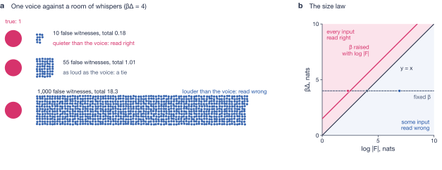
Now keep fixed and let the crowd grow. With and 40 other towns the children hold 80% of the weight; with 4,000 other towns they would hold under 4% (our arithmetic), because each of the many low scorers still gets a little weight (Figure 1b). To keep the true answers on top as the crowd grows, must grow too. Chapter 5 turns this into a theorem with an exact rate, the logarithm of the size of the crowd.
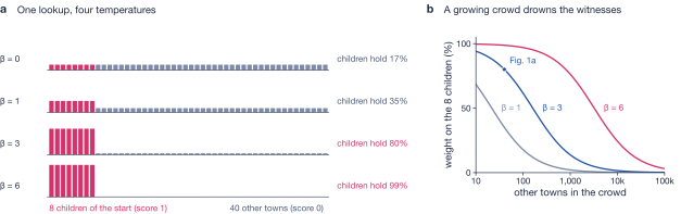
Two more words. The scores before the softmax are called logits. Quantities measured in natural logarithms are in nats: a margin of 3 nats between two logits means one option is times more heavily weighted than the other at .
Graphs, walks and matrix powers
A directed graph is a set of vertices joined by one-way edges; the paper draws vertices as towns and edges as one-way roads. A walk is a sequence of roads, each starting where the last one ended, and may visit a town more than once. A path in the strict sense (a simple path) never revisits a town. A graph with no walk that returns to its start is acyclic; a directed acyclic graph is a DAG. Town is reachable from town if some walk leads from to ; breadth-first search (BFS) finds every reachable town by exploring one road at a time.
The adjacency matrix of a graph with towns is the table with if there is a road and 0 otherwise. The entry of the product is
and each term is 1 exactly when there is a road and a road . So counts the walks of two roads from to , one for each middle town , and counts the walks of roads (Figure 2). The identity matrix counts the walk of zero roads from each town to itself, so counts walks of every length; on a DAG the sum stops, because no walk is longer than the number of towns.
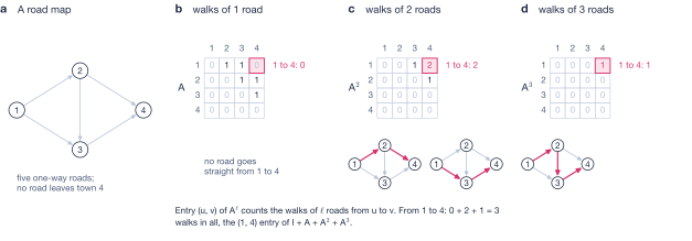
Two variations will matter. First, if you only care whether a walk exists, replace every positive count by 1. Write for 1 if the statement inside holds and 0 otherwise: says “ is within one road of “, and the thresholded product says “within two roads”. Second, repeated squaring: squaring the relation “within roads” gives “within roads”, so squarings reach roads, where adding one road at a time would take steps. This doubling is the heart of the depth law in Chapter 3.
The card game SET
SET is played with 81 cards. Each card has four attributes: a number of symbols (one, two or three), a shape (oval, diamond or squiggle), a fill (solid, striped or open) and a colour (three colours; this tutorial’s own diagrams draw them rose, blue and violet). Every combination appears once, so there are cards. Three cards form a set when, for each attribute, the three cards are all the same or all different (Figure 3a).
There is a neat way to say this with arithmetic. Write each attribute’s values as 0, 1 and 2 and add modulo 3, on a clock with three hours where 3 is back to 0. Three equal values add to , which is 0 modulo 3. Three different values are 0, 1 and 2, which add to 3, also 0. Two alike and one different add to with , never 0 modulo 3. So three cards form a set exactly when they add to zero in every attribute (Figure 3b). The cards with this addition are written , “four copies of the integers modulo 3”.
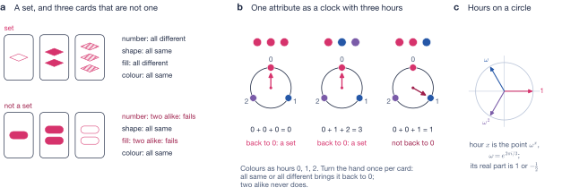
Two facts follow. Any two cards and have exactly one third card that completes a set with them, . And a card in your hand splits the other 80 cards into 40 partner pairs , each of which completes a set with .
The paper’s SET task works like this. A deal is one card in hand and a table of 8 other cards, all distinct, and the question is whether two table cards complete a set with the card in hand. Half of the deals have such a pair. With 8 table cards there are pairs to consider. Larger tests use tables of 16, 20 and up to 40 cards: 40 is the largest table with no pair that completes a set with the card in hand, since such a table holds at most one card of each partner pair.1 Background. In the ordinary game, which asks for any set among the table cards, 20 cards can avoid every set. The paper’s question is narrower: only sets that include the card in hand count. Two kinds of generalisation are tested: to new cards in hand, never held during training, and to larger tables.
2Witnesses: what a layer sums over
This chapter introduces the paper’s central idea: every layer it studies adds up weights over a family of witnesses and reads the total at a temperature. We start with three layers, then define families, the partition function, gates and read-outs, and end with the first rows of the paper’s table of layers.
Lookup, join and pair layer
A lookup is ordinary attention: the query scores each token on its own, , and averages. A join scores combinations. The simplest, 2-simplicial attention3,8, scores every ordered pair of tokens with one number that depends on all three tokens, a trilinear score, and averages a value built from both partners (such as , their entrywise product) over all pairs:
Compare a pair score that splits into two lookups, . Its exponential factors, , so the sum over all pairs is a product of two sums over single tokens: nothing a lookup could not do. The trilinear score does not split this way, so the layer must list all pairs for each query. The number of tokens one score combines is the layer’s arity: one for a lookup, two for this join.
A third kind of layer keeps a pair state: a vector for every ordered pair of tokens , read as “what the model believes about the relation from to “. A pair layer updates from and for every middle token , so its basic witness is a two-step walk (Figure 4). Chapter 3 writes its equation.
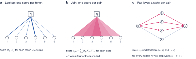
Look at SET. A lookup asks each table card, alone, how promising it is given the card in hand; by the index-card problem, that card would have to know in advance which other cards it pairs with. A join asks every pair at once, and a pair that completes a set can score high as a pair. In search, a lookup asks each town alone how relevant it is to the start; a pair layer can ask about each two-step route start goal.
Families of witnesses
A witness is a small object made of parts: a single token; a pair of tokens; a walk, whose parts are its roads; a subset of tokens; a spanning tree of a graph (a set of edges that connects all vertices without forming a cycle), whose parts are its edges. For each query , a layer has a family of candidate witnesses: single tokens for softmax attention, ordered pairs for the 2-simplicial join, two-step walks for a pair layer. Later chapters add walks of every length and subsets.
The partition function
Every layer in the paper follows one recipe. Give each part of each witness a positive weight , its potential. Multiply the potentials of a witness’s parts to get the witness’s weight. Add the weights of all witnesses in the family: the total is the family’s partition function , a name from statistical physics, where it is the sum of the weights of all states of a system. If each witness also carries a value , add weight times value as well, giving :
Because a weight is a product over parts, its logarithm is a sum: a witness’s score is the sum of its parts’ scores, and potentials are usually exponentials, . Softmax attention is the simplest case: each witness is one token with potential and value , and its output, Equation (1), is .
Gates
A gate is a positive weight that multiplies what passes through a layer. Two kinds appear in this tutorial. A sigmoid gate lies between 0 and 1, like the gates of an LSTM. An exponential gate compares a score with a level : it is at least 1 when and shrinks by a factor for every unit the score falls below the level. The two are related: when is very negative, , so in its low tail, where candidates that do not qualify sit, a sigmoid gate behaves like an exponential one.2 Background: , and when is very negative. The paper’s third principle, below, is about exponential gates.
Read-out links and temperature
Having computed (and ), a layer turns them into its output through one of four links:
- The average is what softmax attention does.
- The count multiplies by a fixed number that may depend on the input size (for example ).
- The OR asks whether at least one witness is present: is near 0 when is near 0 and above 0.95 once . It is the “noisy-OR” of probability: if witnesses are present independently with small probabilities , the chance that at least one is present is , close to 9.
- The free energy is a soft maximum of the scores: with it tends to as grows (Background; Mensch and Blondel10 use this smoothing for dynamic programming). If the scores are minus costs, the same quantity with signs flipped is a soft minimum of the costs: for costs 3, 5 and 6 it is 2.83 at and 3.00 at (our arithmetic). This is how sums of exponentials become the minima of shortest-path algorithms.
The temperature is the scale of the log-potentials. As Chapter 1 showed, it decides whether the best witnesses dominate the total or drown in the crowd.
The paper’s Figure 1
Paper Fig. 1 (Figure 5) shows the three kinds of sum on one search question and one SET deal, with hand-set layers and nothing trained.
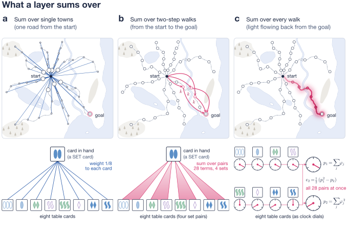
The layer zoo, first rows
The paper collects its layers in one table. Here are the three rows we can read now; Chapters 3 and 4 add rows, and Chapter 7 prints the whole table. A closed form is a formula that computes without listing the family’s members. Cost counts operations for all queries of a sequence (or, for a pair state, all pairs).
Table 1 | The layer zoo, first rows (from the paper’s Table 1).
| Layer | Family | Closed form of | Cost | Read-out |
|---|---|---|---|---|
| Softmax attention | single tokens | a sum | average | |
| 2-simplicial join | ordered pairs of tokens | none (listed one by one) | average | |
| Pair layer, sum over | two-step walks | matrix product | count, scale |
Softmax attention sums terms for each of queries. The join’s trilinear score must be listed pair by pair, pairs for each of queries. The pair layer’s sum over , for all pairs at once, is a matrix product, operations. AlphaFold’s triangle update1 belongs to this family of two-step walks.
Three principles
From this view the paper draws three principles, two of them hypotheses and one a theorem.
- Match the family (a hypothesis). In one step, a layer computes a read-out of its family’s partition function and nothing else; any other structure the answer needs must already be in the partners’ states. So, the paper hypothesises, a layer learns a task easily when the answer is a read-out of its family’s partition function.
- Use a closed form (a hypothesis). A product sums over subsets, a matrix inverse over walks, a determinant over spanning trees. A layer with such a closed form, the paper hypothesises, learns what stacked layers learn by composition, at less cost. Closed forms are parallel computations, so they also mark where a layer must instead loop (Chapter 6).
- Read the sum at low temperature through exponential gates, with a margin that grows with the logarithm of the family’s size (a theorem: the size law of Chapter 5).
The paper checks the size law in Lean, together with the construction half of the depth law. Lean is a programming language in which a proof is written so that a computer checks every step down to the axioms11; Mathlib is its library of formalised mathematics12. The experiments test the first two principles.
Check your understanding
- What is the family of witnesses of softmax attention, and what is its read-out link?
- In the two-step-walk example, why is equal to ?
- Why does a pair score give nothing a lookup could not, while the trilinear score of Equation (2) forces the join to list all pairs?
- Which link asks “is there at least one witness?”, and why does it saturate?
- A sigmoid gate never exceeds 1. In what sense can it still act as an exponential gate?
3Learning to search
Search is where the gap between lookups and pair layers is widest, and where the paper’s new propagator layer does its most striking work. The chapter follows the paper’s argument: Transformers fail, a pair state learns, the depth law says how far it sees, and one propagator layer sees all the way.
The benchmark
The paper uses the search benchmark of Saparov et al.5, with its authors’ generator, test sets and Transformer code. A question is a DAG written as a list of its edges in random order, followed by a start vertex, a goal vertex and the path taken so far; the answer is the next vertex on a path to the goal. Think of standing at a crossroads with a list of one-way roads in your hand.
A question’s lookahead is the number of steps needed to tell the correct branch from the others. On the 250-vertex question of paper Fig. 4d, for example, each town on the answer route, taken as the current town, has as its lookahead its number of roads to the goal. The question of paper Fig. 1 has lookahead 6. Graphs of vertices have lookaheads up to , which is 124 at 250 vertices. Training questions come from a balanced generator, the test sets hold equal numbers of questions at every lookahead, and the benchmark also has random graphs. A run converges when its training accuracy is at least 99.5% on two consecutive checks.3 Training accuracy counts any valid next vertex; test accuracy counts the single next vertex on the shortest useful path, which is unique in every test question, and no test question is trained on.
Transformers do not learn this search as graphs grow
The benchmark’s Transformer, run from its authors’ code with every step of the path asked about, converged in none of ten runs on graphs of 31 to 100 vertices, each trained on at least 5.2 million examples.4 Three more runs were registered for 15 million examples, that is, written down with their predictions, budget and stopping rule before they ran, and were stopped for cost at 2.1 to 3.1 million, still at chance. Every design in the paper was registered this way; the paper lists each prediction with its outcome. Its authors trained it on 236 million examples per run on a variant that asks only about the first step: 5 of 14 seeds converged at 31 vertices, 2 at 41 and 1 at 49.
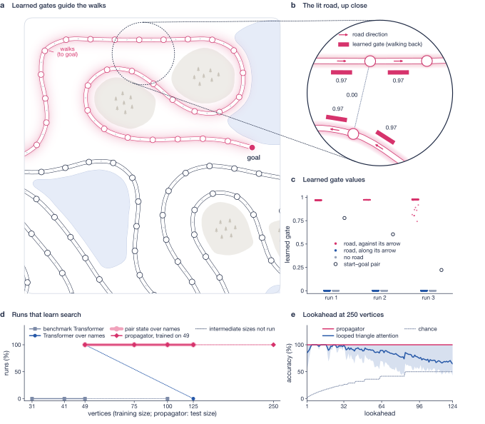
Do the paper’s models win only because they read the graph better? To check, the paper trained a fair control: a Transformer given the same vertex representations as its own pair models, with the starting features of each pair of vertices added into its attention and read-out. It converged in all three runs at 49 vertices and in none of three at 125, within 10 million examples (Figure 11d).
Why a lookup must precompute reach sets
Stand at the current vertex and consider a child : the right move is to the child from which the goal can be reached. In one attention step sees only ‘s key, filed before the question was asked: the index-card problem. So ‘s state must already say whether the goal is reachable from , for whatever goal the question names, and the only way to have that ready is for each vertex to carry the set of vertices it reaches. That is what trained Transformers do: Saparov et al.5 found that each vertex holds its reach set and successive layers merge these sets. In witness terms, the answer is a sum over walks, and a layer over single tokens can answer only if each token has already computed those walks. The sets grow with the graph, and fewer and fewer training runs converge.
A pair state learns
The paper’s pair models first turn the tokens that mention a vertex into one vector for that vertex, its name, and start each pair’s state (16 numbers) from learned features of the two names. Then each summed pair layer applies
Here is the state rescaled to unit size over its 16 channels, the same after the first update, , and learned matrices ( always marks learned weights), a sigmoid gate, entrywise multiplication, and the MLP a small network applied to each pair separately. The heart is the sum over the middle vertex , something about times something about : a matrix product over two-step walks.
Eight such layers, with 39,000 to 49,000 parameters, converged in all twelve runs on graphs of 49 to 125 vertices, each within 1.3 million examples, and each answers at least 98.6% of test questions at every lookahead (Figure 11d).5 Stopped at convergence they answer only 65 to 91% of the benchmark’s random graphs, because balanced training rarely asks about later steps of a path or paths that merge; trained on to 3 million examples, as the propagator below is, they answer 96.6 to 97.5% at 49 vertices.
Three more ways to sum over the middle vertex
The paper compares the summed layer with two relatives that change only the sum over (Figure 6).
- Triangle attention2 replaces the equal weights by a softmax over of a score that couples the two legs:
Because each score involves both and , it must form and store all scores.
- The OR join gives each leg its own sigmoid gate and reads the sum through the OR link, one matrix product per channel:
A layer is looped when one block, with one set of weights, is applied times in a row; the paper’s looped models draw from 5 to 8 during training and are tested after iterations.
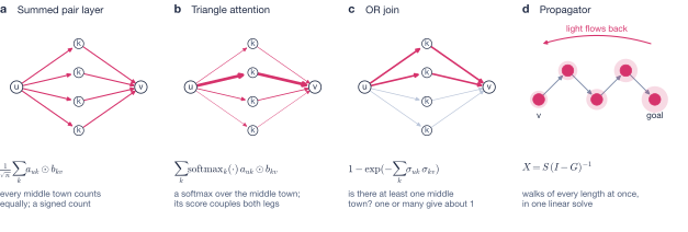
The depth law
How far along a graph can pair layers see? Repeated squaring suggests an answer, and the paper proves it in both directions.
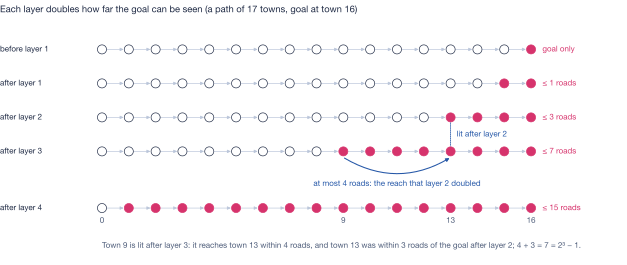
The construction. Give the pair state a channel that starts as “within one road” and a channel that starts as “this vertex is the goal”. Each layer squares through the sum over , so after layer , says “ is within roads of “. Each layer also updates the goal channel: is marked if it is within roads of a vertex marked one layer earlier. Since , after layer the goal channel marks exactly the vertices within roads of the goal (Figure 7). A small MLP with thresholds keeps every channel a clean 0 or 1, and a last unit checks that is a child of the current vertex .
The lower bound. Could a cleverer network of the same kind see further? A message-passing network is a graph network in which each vertex repeatedly updates its state from its own state and the collection of its neighbours’ states. The classical tool for its limits is the Weisfeiler–Leman test: give every vertex a colour, then repeatedly recolour each vertex by its own colour together with the collection of its neighbours’ colours. Two vertices that still share a colour after rounds cannot be told apart by any message-passing network of depth that starts from the same colours.6 Background: a network of this kind sees exactly what the colours see, round by round. The folklore 2-dimensional version colours pairs of vertices: the new colour of is its old colour together with the collection, over all middle vertices , of the colour pairs . That is the shape of the pair update, so after layers a pair’s state can depend only on its colour after rounds13. If two questions give the pair the same colour, no -layer network of this kind can answer them differently.
The paper builds two directed paths. In one the goal lies roads beyond , so it is reachable; in the other it lies roads behind and , upstream, so it is never reached (Figure 8). It proves that gets the same colour in both, for every .
Why, for every : a window and a census. The proof pins down exactly what rounds can know. After rounds of folklore 2-WL on a path, a pair knows three things and nothing more: how far apart and are, and in which direction, if they are at most roads apart; every label (the goal, the current vertex, an end of the path) within roads of or of , a window of radius around each end of the pair; and one count over the whole path, the census: how many vertices see each possible small window of labels around themselves. For the pair after rounds, the window runs from roads before to roads after it. A goal roads beyond sits just past its right edge, and a goal roads behind just past its left edge. If the path is long enough and is far enough from both ends, the two paths also have the same census, so the two questions look identical from . Move either goal one road closer and it enters the window, and the colours differ: the bound is exact.7 The census is where the length of the path enters: on paths that are too short, or with too close to an end, it can differ between the two questions.
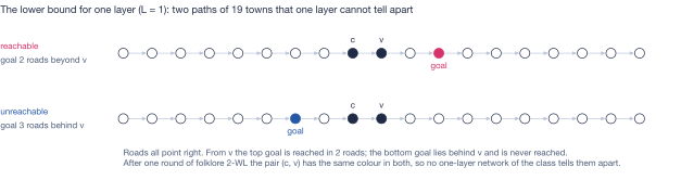
Here is the theorem, in the paper’s terms with lightly simplified wording.
Theorem 1 (Depth law)
(i) For every number of vertices and every there are weights for layers of Equation (5), applied to the state itself rather than its rescaled copy, whose read-out at is positive exactly when is a child of from which the goal is reached in at most steps. (ii) Let each of layers update by any function of and the collection , and let every pair start from a state that depends only on its atomic type (whether , which roads join and , and which of them is the goal or the current vertex). For every , no such network separates at a goal steps beyond from one steps behind it, both goals on a directed path of vertices.8 The paper’s Proofs give the general condition: at least vertices, with at least steps after the first vertex and at least steps before the last. So, from such anonymous starting states, the largest distance from to the goal that layers decide on every graph is exactly .
Lean PairSearch.pair_states_search_sharp, PairSearch.pair_states_search_looped
Part (i) is repeated squaring, a classical idea14, checked in Lean for the layer’s own form.9 The construction uses five channels and residual ReLU MLPs of width 4; its first layers are one repeated layer. Part (ii) is the window-and-census argument above, a written proof (not in Lean), and the paper’s exact colour refinements for agree with it. It does not cover starting states that identify vertices, such as the trained models’ names: with unique names, two rounds of an update that keeps all its information already see the whole graph. The summed pair layer, triangle attention and the OR join all belong to the class of part (ii). The propagator, below, does not.
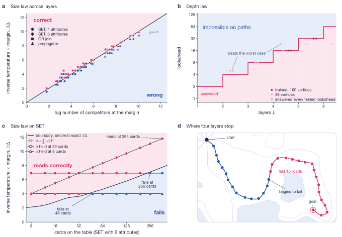
What trained models do. Lookahead counts from the current vertex, one more than from its child, so part (i) guarantees lookahead and part (ii) rules out for anonymous states on paths. Trained pair states over names, with from 2 to 8 layers, answer at least 95% at every lookahead up to in every run and fall soon after (Figure 9).10 Depths 2 to 8 at 49 vertices and 4 to 6 at 100. At 100 vertices four layers answer 28 to 36% at lookahead 17 and five layers 18 to 58% at 33, cut-offs registered in advance. A few models beat the worst case: the two-layer models answer lookahead 5, and two four-layer runs at 49 vertices that never converged answer 87 to 98% beyond lookahead 16.
Why do models that do have names still stop near ? The paper proves no reason and calls the match empirical. Its Supplement reports what the trained states hold: a linear probe (a linear regression on the 16 channels) recovers “ reaches the goal within 32 steps”, the construction’s goal channel, with an AUC of 0.97 to 1.00 (1 is perfect, 0.5 chance) after the fifth iteration of a looped pair layer; and an eight-layer model’s read-out, applied after each layer, answers at least 90% only up to lookahead 1 for five layers, then up to 5, 9 and 24 (the deepest tested) after layers 6, 7 and 8. The paper claims no more than that.
One layer for walks of every length
Eight pair layers spend their depth composing two-step walks. The second principle says: if the family has a closed form, use it. The family of walks of every length has one.
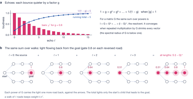
From echoes to matrices. Clap at one end of a long hall: you hear the clap, then an echo quieter by a factor , then an echo of the echo, quieter by , and so on. The total is the geometric series
5 when (Figure 10a); if the sum never settles. The same identity holds for matrices. Let be an matrix of gates, the fraction of weight that passes from to in one step. Then adds up all walks of steps, each weighted by the product of its gates, exactly as counted walks, and
The matrix is the resolvent of . The series converges when repeated multiplication by eventually shrinks every vector, that is, when the spectral radius of (the largest size of its eigenvalues) is below one. Then one linear solve, about operations, replaces infinitely many walks.
The propagator. In each of four channels the paper’s propagator forms gates and a source from the rescaled pair state , caps the gates, and solves for the walk sum:
with and , , , learned. Every quantity is an matrix indexed by pairs of vertices. Take one row: if the source is 1 at the pair (current vertex , goal) and 0 elsewhere in row , then , the total weight of all walks from the goal to through the gates. The logarithm of and then enter the pair state through a learned map and a gate, followed by the per-pair MLP. The first fraction in Equation (6) is the row cap: if the gates leaving a vertex add up to more than , they are scaled down to add up to exactly .
Why the cap works. If every row of a non-negative matrix sums to at most , each step passes on at most a fraction of the weight, so all walks of steps from any vertex carry at most , and the series converges like on any graph, cycles included. The general statement is Gershgorin’s circle theorem15: every eigenvalue lies in a disc around a diagonal entry whose radius is the sum of the sizes of the other entries in its row, so the spectral radius is at most the largest row sum of the entries’ sizes.
How the layer searches. Set the gates by hand: open on every road walked backwards (a gate on when there is a road ), closed elsewhere, with the source on the goal. Weight starts at the goal and flows backwards along roads, reaching exactly when a road path leads from to the goal. So exactly when the goal can be reached from , and a walk of roads keeps weight (paper Fig. 1c, Figure 10b).
The propagator was the third registered design: the fixed and the row cap were added after two earlier designs without them lost accuracy at 250 vertices, the first (which learned ) in one of three runs and the second (every channel started near one) in two of three, where the spectral radius passed one. A ceiling well below one would cost accuracy on long routes, since a walk of steps keeps at most of its weight (Chapter 5).
Results. Trained on balanced graphs of up to 49 vertices, the propagator layer of 28,472 parameters converged in all three runs within about a million examples, each run training for 160 to 188 seconds on one H100 GPU. In every run it answers every test question at every lookahead at 75, 100, 125 and 250 vertices (at 250 vertices, 200 questions at each of 124 lookaheads), and 99.0 to 100% of the benchmark’s random graphs of that size. Looped triangle attention, trained to the same sizes, answers at least 99% at every lookahead at 250 vertices in one run of three, and in four of fifteen runs across five training variants (Figure 11e).
What the trained layer learned. Each trained run recovers the hand-built layer plus one extra gate (Figure 11a–c). On a 250-vertex question, the answer channel’s gates after the cap are 0.97 to 0.98 (median) on reversed roads and below on forward roads and on pairs with no road, low enough: the hand-built capped layer still answers correctly with gates up to on those pairs.11 Without the cap the limit would be , where is the total weight of all walks along the road gates; at that background the walk sum diverges. The source sits on the pair of the current vertex and the goal (0.999), so walks start at the goal. The extra gate, on the question’s own start and goal (0.22 to 0.78 across runs), is closed in the construction.
Cost and precedents. One training step of the propagator (without the cap) processes 6.0 and 6.9 times as many examples per second as a looped OR join (in its simplest, one-term form) at 125 and 250 vertices, with 0.39 and 0.52 of its memory. Earlier models compute resolvents, fixed points or path sums over a given graph16–18; none that the paper found computes one from gates on a pair state, or applies one to search. Table 2 adds this chapter’s four layers to the zoo.
Check your understanding
- Why must a Transformer build reach sets in its token states, while a pair state need not?
- By the construction, how many roads from a child can three pair layers see, and what lookahead is that?
- What does the Weisfeiler–Leman argument add, and why does it not apply directly to the trained models?
- Why does the propagator need the spectral radius of below one, and how does the row cap ensure it?
- In a trained propagator, which gates are open and where is the source? Why does that answer the question?
Table 2 | Rows added in this chapter (from the paper’s Table 1). Cost for all pairs.
| Layer | Family | Closed form of | Cost | Read-out |
|---|---|---|---|---|
| Triangle attention | two-step walks | none (listed over ) | , memory | average |
| OR join | two-step walks | matrix product | , memory | OR |
| pair layers, or one looped times | walks of at most steps | repeated squaring | OR, threshold | |
| Propagator | walks of every length | one solve, | OR, free energy |
4Learning SET
SET is the paper’s second test case. Its witnesses are pairs of table cards, so single tokens are the wrong family, and its rule is arithmetic modulo 3, so one can see exactly what each trained layer computes. This chapter builds three tools along the way: characters, Newton’s identities and the Jacobi–Anger expansion.
Transformers memorise before they learn
A four-layer Transformer of 535,000 parameters trained on 32,768 deals answers 98% of its training deals and 54% of new ones, and first passes 90% on new deals at 524,288 deals (Figure 15a). Given enough distinct questions it does learn the rule: trained with 27 different cards in hand on 221,184 deals, a four-layer Transformer of 66,000 parameters answers 93% of deals whose card in hand it never held. With fewer cards in hand in training, every model the paper trained, the join included, is at chance on new cards in hand.
No lookup can rank SET’s pairs
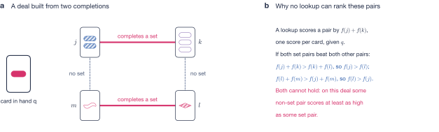
Suppose a layer scores each pair of table cards by adding two lookup scores, one per card: , where may be any function of the card in hand and one table card. This is the index-card problem in its purest form: each card’s score is fixed before its partner is known.
Proposition 1 (No single-card scores rank SET’s pairs)
Let a layer score each pair of table cards by , the sum of two lookup scores, for some function of the card in hand and one table card. For every , every and every table size there is a deal on which a pair that does not complete a set with scores at least as high as a pair that does.
The proof is a small trap (Figure 12). Take any card and its completion , then another card and its completion . The pairs and complete sets; the cross pairs and do not, because each card has exactly one completion. If both set pairs scored above both cross pairs, the first comparison would give and the second . Both cannot hold. Separations of this kind between pair-based and single-element set networks are known in general19.
The join learns, and computes with clocks
A join’s family is the pairs of table cards, so Proposition 1 does not bind it. One layer of 2-simplicial attention with 62,000 parameters passes 90% at 8,192 deals, 64 times fewer than the large Transformer needs, and trained on 55,296 deals it answers 99.6% of deals with new cards in hand.
What does it compute? In this tutorial a clock always means one thing: a rule that reads an hour (0, 1 or 2) and scores it by , which is 1 at hour 0 and at hours 1 and 2. (A trained clock may be turned by a fixed angle, a mix of that cosine and the matching sine; the counting box below shows that either way it is one conjugate pair of characters.) For SET, the natural hours are the four attributes’ values of the sum : hour 0 on an attribute means “all the same or all different” there.
The paper decomposes the trained join’s score, over all triples of cards, into patterns, and finds that in joins trained with all 81 cards in hand, 82 to 94% of the score’s variance lies on just four clocks, one per attribute (Figure 15b). “Variance lies on a pattern” means this. Any score over the three hours of one attribute splits into its average plus a varying part, and the varying part is a mix of a cosine and a sine of . Scores of 2, 0.5 and 0.5 at hours 0, 1 and 2, for example, are their average 1 plus , which is exactly the clock: all of their variation lies on it. The join’s score for a pair is, to a good approximation, the sum of its four clocks.
Then the softmax turns the sum into a product. Writing for the four clock values,
Each factor is large only when its attribute is at hour 0, so the product is large only when all four are, that is, when the three cards form a set: the softmax turns four clocks into an AND. In the trained join of Figure 15b, the softmax weights over the 81 possible third cards peak on the set, and the next largest weight is .
Counting with characters
To count sets exactly, we need a little algebra on the cards. A group is a set with an addition that has a zero and can be undone (every element has a negative); SET’s cards with addition modulo 3 form one, and the order of addition does not matter, so it is an abelian group. Its characters are the group’s version of the waves of a Fourier series (which writes a function as a sum of waves): functions that turn each card into a point on the unit circle and turn sums into products.
Newton’s identities
Counting with characters needs, for each character, a sum over all pairs of table cards of a product of per-card factors, and listing pairs costs terms. An identity that Isaac Newton found more than three centuries ago removes the listing. For numbers , the elementary symmetric polynomial is the sum over all subsets of of them of their product, and the power sum is . (Here with a subscript is a polynomial, not Euler’s number .) Newton’s identities20 give the first from the second:
Newton attention as a layer
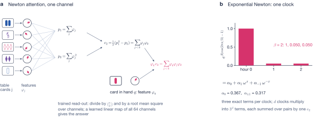
Newton attention, one of the paper’s three new layers, puts this to work (Figure 13a). It has 64 channels, copies of the same computation with their own learned weights. In each channel:
- Each card gets a complex feature , a dial: a sigmoid gate between 0 and 1 times a point on the unit circle at an angle learned from the card’s vector.
- For each card, the layer adds up its partners’ features and their squares, and over the other cards, and forms and .
- The card in hand , whose partners are the table cards, multiplies in its own feature: , one product per triple of card in hand and pair of table cards.
- As trained, the features for are divided by , so that becomes an average over pairs, then by a root mean square over the 64 channels computed for each deal, and a learned linear map turns them into the answer.
If each dial is a character, step 3 gives , and summing over characters counts sets:
Proposition 2 (Characters count set pairs at linear cost)
Let be the card in hand and the table cards. There are 40 characters of , one from each conjugate pair of non-trivial characters, such that for every and every table the number of unordered pairs of table cards that complete a set with is
Lean Newton.set_count, Newton.newton_identities
The trivial character contributes and each conjugate pair twice the real part of one member, as in the counting box. Each costs two power sums, so the count costs time linear in per channel. Measured on a GPU, Newton attention’s time and memory per training step stay flat from 9 to 4,096 tokens per sequence, while the join runs out of memory at 1,024 (Figure 15d).
What Newton attention learned. Trained as the join is, a Newton layer of 55,714 parameters first passes 90% at 32,768 deals, four times as many as the join needs. In all 17 runs that reach 97%, its channels hold 38 to 40 of the 40 characters of Proposition 2. That explains the slower learning: the join’s exponential turns four clocks into the AND over all 81 characters for free, while Newton’s read-out is linear in each channel and must find the 40 characters one by one.
Why it failed on larger tables. Read out as trained, the layer answers only 73 to 76% on tables of 16 cards. The divisions of step 4 are the reason (Figure 14). Measure the read-out’s decision threshold in sets: trained at 8 cards, it calls “set” once its output passes the value it gives a deal with 0.54 sets, between no set and one set, as it should. From 8 to 16 cards one set’s term shrinks by and the root mean square by 0.44, so one set’s normalised share falls to about half, while the normalised baseline of the other pairs grows 2.3 times. A model of these two divisions, fitted on 8-card deals alone, predicts that the same threshold sits at 1.76 to 1.79 sets on 16 cards; the measured value is 1.76 to 1.77. A deal with exactly one set now falls below the threshold and is called negative.
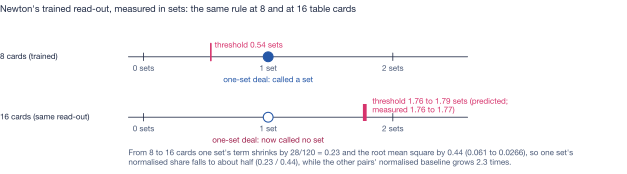
The fix is to train at two sizes: trained on both 8- and 12-card tables, the same layer answers at least 95.5% at 16 cards and 92.8% at 20 (92.4% at 16 in a repeat with the same seeds). From two sizes it learns a threshold that depends on size. Read as a count, with no division, the layer is exact at every size, but that form did not train to the rule (85% on 8-card tables). Chapter 5 turns this into a general lesson.
Exponential Newton: the join’s softmax at Newton’s cost
Can one keep the join’s sharp softmax, which gets the AND for free, and Newton’s linear cost? The paper’s third new layer, exponential Newton, does this exactly when the join’s score is a sum of clocks on and the layer is given the modulus 3, told that hours wrap around after three, where the join learns its clocks from data.
The trick is that the exponential of a clock takes only two values, so it has an exact three-term Fourier series. With hour and score , which is 0 at hour 0 and at hours 1 and 2, write . The exponential is 1 at hour 0 and at hours 1 and 2, and
Check: at the right side is ; at it is , using . This is the Jacobi–Anger expansion of as a Fourier series21, folded onto three hours.
For clocks, multiply such expansions: each term of the product is a character times a fixed coefficient, so there are channels, and because a character splits over the three cards, each channel’s sum over pairs of table cards is one Newton .
Proposition 3 (Jacobi–Anger on )
For every and ,
with and as above. Hence, for a join whose score on the card in hand and table cards and is with clock hours , the partition function and output of the softmax over the distinct pairs of table cards are sums over channels of Newton’s , computed in operations.
Four clocks give all 81 characters, with weights fixed by (Figure 15c). The same expansion works for any finite abelian group, at a cost of the group’s size times , provided the group is given. In the trained layer each clock is a learned rule that reads an hour off each card (as a probability over the three hours), with one learned .
Results. Trained as the join but with the modulus given, exponential Newton with four clocks first passes 90% at 8,192 deals, the join’s budget, and answers 69% at 2,048 deals against the join’s 51% (Figure 15a). But in 10 of 12 models the four learned clocks read one attribute twice and another not at all. Their errors on larger tables fall on deals holding a pseudo-set, a pair that completes a set on the three clocked attributes but not the fourth, and so scores exactly as high as a true set: a zero margin, which no temperature fixes (Chapter 5). With six clocks the layer has channels (not to be confused with the 729 cards of Chapter 5’s six-attribute SET), and 5 of 6 models covered all four attributes. The six-clock layer passes 99% at 8,192 deals (99.9% and 100.0% in two repeats of the job with the same seeds). Trained on 8-card tables, it answers at least 97% of deals with new cards in hand on 16- and 20-card tables, for each of three seeds in both repeats, at its trained temperature (Figure 15e).12 This is with the learning rate chosen on held-out cards in hand. With the rate picked on the training cards in hand, the registered test failed: one seed scored 52.3%.
Two limits belong here. At SET’s table sizes is larger than the pair terms it replaces (with 8 cards there are only 28 pairs, against for four clocks), so the saving is for long sequences, where the paper has not timed it. And the layer is given the group, which the join learns.
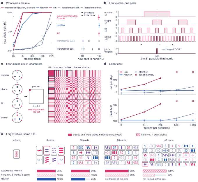
Table 3 | Rows added in this chapter (from the paper’s Table 1). Cost for all queries; Newton’s power sums are computed once and shared by every query.
| Layer | Family | Closed form of | Cost | Read-out |
|---|---|---|---|---|
| Newton attention | -subsets | per channel | count; trained as a mean | |
| Exponential Newton | unordered pairs, clock scores | characters | average |
Here means “the coefficient of in the multiplied-out product”, the generating function of the worked example above.
Check your understanding
- In Figure 12, write out the two inequalities that a sum of single-card scores would need, and show that they contradict each other.
- Use Newton’s identities to compute of from its power sums, and check by listing the pairs.
- How many characters does have, how many conjugate pairs, and how many characters make up the four clocks? Why can the join get by with four clocks while Newton attention needs 40 characters?
- Why did Newton’s mean read-out fail on 16-card tables, and why does training on two table sizes fix it?
- A trained exponential Newton layer clocks number twice and never clocks colour. Why can no temperature rescue it on large tables?
5Temperature and size: the size law
Chapters 3 and 4 showed layers that keep working on inputs much larger than any in training, and layers that break. This chapter explains the difference with the paper’s second theorem, the size law, and then shows it measured.
One voice against a room of whispers
Many questions here are existence questions: is there a walk from this child to the goal? Is there a pair on the table that completes a set? Suppose a layer answers by scoring every candidate witness and adding up exponential gates. Call a witness true if its score is at least a level and false if its score is at most , where is the margin. Measure each gate relative to the level:
Two facts follow at once. If some witness is true, its own term is at least and all other terms are positive, so . If no witness is true, every term is at most , so , where is the number of candidates. That second step is a union bound: a sum of many small terms is at most their number times the largest. So if , the threshold ““ separates the two cases; taking logarithms, (Figure 16).
The bound is also tight. An adversary can put every false witness exactly at the margin, so that their whispers add up to exactly , while a true input can have just above 1, with one witness at the level and the rest far below. If the false input is louder than the true one, and no threshold separates them.
Theorem 2 (Size law)
Let be a finite nonempty family with scores , a level , a margin and , such that every witness is true, , or false, . Let . If , some witness is true exactly when . If no witness is true, , with equality when every score is . Hence, for and scores free within the margin, some threshold on decides existence on every input if and only if
with the strict threshold at equality. Under the same condition, when a true witness exists, the softmax weight on the true witnesses is at least one half.
Lean Framework.size_law_iff, Framework.size_law_equality, Framework.gated_existence, Framework.gated_existence_log, Framework.background_le, Framework.tight, Framework.softmax_existence
The whole theorem is checked in Lean: both directions of the “if and only if”, the equality case and the softmax statement. For single tokens the law restates a known requirement, that attention logits must grow with the logarithm of the sequence length22–24. What the paper adds is the statement for families of witnesses and its worst-case tightness.
What the law says for each family
The required temperature depends on the family’s size:
- Single tokens: , so must grow like .
- Ordered pairs: , about , so must grow like , twice as fast.
- Subsets of : about .
- Walks of every length, without the row cap: the total walk weight of the road gates takes the place of , and a witness of steps whose gates are each carries only , so the margin also pays a path-length cost, . A gate ceiling well below one therefore costs accuracy on long routes.
Exponential gates against cancellation
There is another way to silence false witnesses: make them cancel. Newton attention’s characters do this; in the one-attribute example of Chapter 4 a non-set pair contributes exactly, and exact cancellation by group characters works at every size. But trained characters are only approximately right. Suppose each false witness leaves a small independent residual of size , positive or negative at random. Random residuals add like a random walk, growing like times the square root of their number, and the paper shows that once there are false witnesses the read-out errs with probability at least . Exponential gates need a temperature that grows like at fixed precision; approximate cancellation needs every term’s precision to improve as the family grows.
Read-outs divided by the number of candidates
A third failure is subtler. A read-out that divides its existence signal by the number of candidates, with its threshold fixed at one size, fails at larger sizes at any precision: one witness’s share of the total shrinks as the candidates multiply. Newton’s mean read-out, trained on 8 cards, answers 73 to 76% at 16 (Chapter 4). The looped pair layer that sums over the middle vertex with the fixed factor , trained at 49 vertices, answers 61 to 73% at 125, averaged over lookaheads.
Not every average fails. Triangle attention averages too, but it divides by the total weight (a softmax), not by the number of candidates, as the softmax half of the size law allows. Layers read through exponential gates, including sigmoid gates working in their low tail, transfer: trained at 49 vertices and tested at 125, the looped OR join answers at least 99.6% and looped triangle attention at least 99.2% at every lookahead; the propagator transfers to 250 vertices; exponential Newton from 8 cards to 20.
The law, measured
The paper tests the law on hand-set layers, nothing trained, where the margin is known.
- The OR join on search. A hand-set looped OR join needs an input gain (the slope of its sigmoid gates, which plays the role of ) rising from 13.5 at 50 vertices to 17.8 at 1,600: growth with the logarithm of the size.
- Exponential Newton on SET. A pair one attribute away from a set has one clock at instead of 0, so the margin is , and the read-out threshold is one half. The rule , for table pairs, makes , so each of the at most false pairs contributes at most , and together at most one half, the threshold, while a true set pair contributes at least 1. With this rule the hand-set layer is exact on tables of 8 to 40 cards, while the temperature that suits 8 cards answers 66.7% at 32 cards. On a larger made-up variant of SET with six attributes ( cards, so tables of up to 364 cards can lack a set), the rule is right to 364 cards, the 8-card temperature fails from 48 cards and the 32-card temperature from 256 (Figure 17c).
The paper then measures the critical , the smallest that answers every question, on 42 instances of four hand-set layers (Figure 17a). The worst case, , lies 1.2 to 4.1 nats above the measured value for the SET layers and the OR join: real inputs are kinder than the worst case. Evaluated on the realised scores, the theorem’s own condition bounds the false total , which is about when competitors sit at the margin and the rest are far below; for SET they are the pairs one attribute away from a set. With in place of , every measured flip lies within 0.3 nats of the line , except the OR join’s beyond 200 vertices (0.8 nats at 1,600). This is a data collapse: four layers on two tasks fall on one line once the axes are chosen right. For the propagator, lies 0.1 to 1.4 nats below the measured value, because its margin also pays the path-length cost.
The law also shaped a trained model. On CLRS-30 (Chapter 6), the trained OR-join block needed its input gates shifted by a learned multiple of : without the shift it came within a point of triangle attention on 8 of 12 tasks, with it on 11.
Check your understanding
- From “a true witness contributes at least 1” and “each false witness contributes at most “, derive the condition .
- If doubles, by how much must grow for a layer over single tokens, and for one over ordered pairs?
- Why does a read-out divided by the number of candidates fail at larger sizes even when every feature is exact? Why does a softmax average not?
- Why does approximate cancellation break as the family grows, while exponential gates hold?
- Why is the SET temperature rule and not ?
6What the principles predict elsewhere
So far the principles have explained two tasks the paper chose. This chapter asks what they predict on a standard benchmark built by others, and on language and chess, where the paper expects pairs to matter little.
CLRS-30 in brief
The CLRS-30 benchmark25 asks networks to imitate 30 classical algorithms from the textbook by Cormen, Leiserson, Rivest and Stein; the paper uses its twelve graph tasks. Models train on graphs of up to 16 nodes and are tested on graphs of 64. The benchmark can supply hints, the algorithm’s intermediate states, as extra supervision; the paper trains without hints, from inputs and final outputs only. Scores are accuracies in percent, and differences between them are in points (percentage points). The twelve tasks:
- BFS and DFS: each node’s parent in the breadth-first and the depth-first search. CLRS’s DFS takes neighbours in index order and restarts from the lowest-numbered unvisited node when it runs out, so its output is the lexicographic DFS forest (a set of trees).
- Topological sort: an order of a DAG’s nodes in which every edge points forward.
- Articulation points and bridges: the nodes, and the edges, whose removal disconnects the graph.
- Strongly connected components (SCC): the groups of nodes that can all reach each other; the output names one representative node per group.
- Kruskal and Prim: two ways to build a minimum spanning tree (the cheapest spanning tree); Kruskal’s output marks the tree’s edges, Prim’s gives each node’s parent in the tree grown from a start.
- Bellman–Ford, Dijkstra and DAG shortest paths: each node’s predecessor on its shortest path from a source. Without hints, Bellman–Ford and Dijkstra have the same test inputs and answers.
- Floyd–Warshall: the predecessor on the shortest path between every pair of nodes. Its answer is a pair.
One small looped block against a large model
The paper’s model is one looped block over a pair state of width 128 (each pair holds 128 numbers), with 186,000 parameters, iterated eight times at 64 nodes. Half of its channels are OR joins. The other half take a power mean over the middle node26,
where and are learned gates; as grows a power mean approaches its largest term, so if the gates are exponentials of minus distances, it picks out the shortest route through . Both halves shift their input gates by a learned multiple of , as the size law asks (Chapter 5). The design was chosen at width 32 on the benchmark’s official 64-node test graphs, confirmed at width 32 on freshly drawn test graphs and new seeds (within a point of looped triangle attention on 10 of 12 tasks), and the width-128 layer was then registered with its predictions and run once.
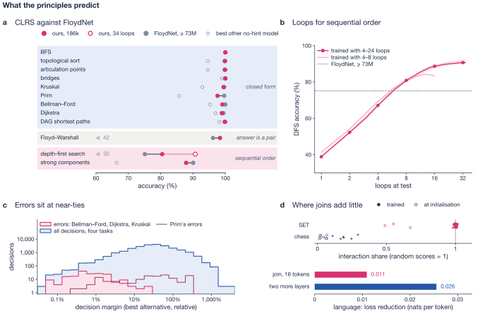
The comparison is FloydNet27, a pair-state network of about 73 million parameters at its smallest depth, trained without hints. On the official test file the paper’s block matches (within half a point) or beats FloydNet on 9 of 12 tasks; it is below on Bellman–Ford (by 0.9 points), Prim’s algorithm (2.1) and strongly connected components (2.2).13 On Dijkstra it is 0.49 points below FloydNet, inside the half-point band by 0.01. On the fresh graphs Dijkstra falls 0.003 points short, which is why the fresh-graph count is 8. Of the registered predictions, matching or beating on at least 8 of 12 tasks, beating FloydNet’s 75.1% on DFS and reaching its 96.2% on Floyd–Warshall held; matching or beating on all 12, reaching 99.0% on Prim and 90.1% on SCC failed (9 of 12; 97.6; 87.9). On 128 freshly drawn test graphs per task it matches or beats on 8 of 12. The comparison crosses protocols: FloydNet’s scores are from its paper (online training, 32 to 80 layers), the block’s from 80,000 training steps on a fixed pool of graphs, three seeds and final parameters.
The cleanest test of the first principle is Floyd–Warshall, whose answer is a pair. The two pair-state models score 96.2% (FloydNet) and 98.3% (the paper’s block), while the no-hint models of Bevilacqua et al.28 and Rodionov and Prokhorenkova29, which keep a state per node, score 40.8% and 42.2%. A node-state model must squeeze a pair-valued answer into single-node states: the index-card problem again.
Parallel and sequential: NC and P
Two tasks, DFS and SCC, need a new idea: problems that can be solved fast in parallel against problems that seem to need a long sequence of steps.
P (not the number of table pairs of Chapter 5) is the class of problems a computer can solve in a number of steps polynomial in the input size . NC is the class that can be solved in polylogarithmic time, a number of steps bounded by a power of such as , using polynomially many processors in parallel. Adding up numbers is in NC: add them in pairs, halving the list each round, and finish in rounds. Every problem in NC is in P; whether the classes are equal is a famous open question, and most researchers believe they are not. A reduction from problem A to problem B is a fast way to turn any question of A into a question of B with the same answer, so that a fast method for B would give one for A. A problem in P is P-complete if every problem in P reduces to it; such a problem has no fast parallel algorithm unless NC = P30.
The closed forms of Chapter 2 are parallel: matrix inverses and determinants lie in NC31, and so do repeated squaring and Newton’s recursion. A layer that applies one of them plus entrywise operations is an NC computation, and so is a stack of polylogarithmically many such layers. Lexicographic depth-first search is P-complete32: deciding whether node is visited before node , when DFS always takes the lowest-numbered unvisited neighbour, is as hard as anything in P. So, unless NC = P, no stack of polylogarithmically many such layers computes it on all graphs, and a looped layer must run more than polylogarithmically often.14 With a technical condition on how the weights may depend on the graph size. The argument does not say how many loops are enough.
SCC’s representative. CLRS finds components with Kosaraju’s algorithm: one lexicographic DFS of the graph, recording each node’s finish time (the moment the search has explored everything below it), then a DFS of the graph with all edges reversed, taking nodes in order of decreasing finish time. The paper shows what the library’s representative is, and how hard it is:
Proposition 4 (The component representative is P-complete)
The representative that CLRS-30 assigns to a strongly connected component is the component’s first vertex discovered by lexicographic depth-first search. Deciding whether a given vertex is the representative of its component is P-complete.
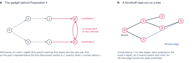
The proof is a reduction from “is visited before ?”. Add two new vertices and , numbered 1 and 2, below every original vertex except the start 0, with roads , and both ways between and (the other vertices are renumbered upwards). Then is a component of its own, and whichever of and the search reaches first steps into it first: its representative is exactly when is visited before (Figure 18a). The paper checks the gadget against the library’s own function on 400 of 400 random graphs. The components themselves can be found in parallel, through reachability; only the representative is P-complete. Topological sort is DFS too, but on acyclic graphs, where lexicographic DFS lies in NC by a result of de la Torre and Kruskal33; the block scores 99.9% on it.
Errors sit where the theory puts them
If the theory is right, the block’s DFS and SCC errors should sit on the parts of the output that depend on the sequential order. They do.
- SCC. Every wrong SCC pointer points inside the correct component: the block finds the components and misses only the representative. Accuracy is 98.8 to 100% where the representative is the component’s smallest index, which a parallel rule finds, and 66.5 to 70.4% where the first DFS pass fixes it.
- DFS. The block is right on every node up to depth 7 in the true DFS tree, and on 67 to 72% of nodes at depths 32 to 63.
- More loops. Trained with 4 to 24 loops instead of 4 to 8 and run 34 times at 64 nodes, the same layer’s DFS accuracy rose from 80.5% to 90.7% (mean of three seeds; 89.8 to 92.4), increasing with each loop up to the training maximum and nearly flat after it (Figure 19b); FloydNet without hints scores 75.1%. This shows accuracy rising with the number of loops. It cannot tell apart how fast the needed loop count grows with graph size: one size, 64 nodes, and 34 loops are consistent with polylogarithmic and with faster growth alike.
- More loops for SCC. The same change on strongly connected components was registered with the prediction that only the order-dependent representatives would gain. Every wrong pointer stayed inside its component and the smallest-index representatives stayed at 98.8%, but the order-dependent ones rose only from 69.0% to 72.8%, within the spread of seeds, and overall accuracy levels off near 14 loops (89.0% at 34, against FloydNet’s 90.1%). The account locates these errors; at this width, more loops do not remove them, unlike DFS’s.
Near ties, and one exception
The remaining errors on weighted tasks sit at near ties, where the margin of the size law is small. A decision’s relative margin is how much worse the best alternative’s path weight or distance is than the true choice’s. On Bellman–Ford and Dijkstra, the median relative margin of the decisions the block gets wrong is 0.5 to 0.6%, against 20.5% over all decisions; on Kruskal’s algorithm the two medians are 1.3% and 42% (Figure 19c).
Prim’s algorithm is the exception. Its errors are not near ties (median 30% against 51% over all decisions), two thirds of them point to the node’s own child (the right tree edge in the wrong direction), and they grow with depth in the tree. The principles do not explain them. The paper tried the family they suggest, spanning trees, through a Kirchhoff read-out. Treat each edge as a wire with a learned conductance (how easily current flows through it); the graph’s Laplacian is the matrix with each node’s total conductance on the diagonal and minus the conductance of each edge off it. Holding the source at zero (grounding) and solving one linear system gives every node a potential; the matrix-tree theorem says the same Laplacian, through its determinant, sums over all spanning trees. With conductance 1 on the true tree’s edges the read-out is exact on all 2,048 official test nodes (Figure 18b). But the trained layer gives confident conductance to edges outside the tree at 64 nodes, and in two registered tests neither the Kirchhoff read-out (97.20%) nor a learned shift of its conductances (96.84%) removed Prim’s errors; without them the block scores 97.57%. Prim remains open.
Where joins add little: language and chess
The first principle also predicts where pair layers should not help: tasks whose witnesses are mostly single tokens.
Language. In an 8-layer language model of 51 million parameters, a join over the previous 16 tokens, added in every second block, gains 0.011 nats per token after 200 million tokens of FineWeb-Edu34; two more ordinary layers gain 0.026 (Figure 19d). The models were trained at one scale, budget and window; joins over long contexts gain more35, a regime the paper did not test.
Chess. In models that pick the solving move of Lichess puzzles, joins beside or in place of attention never gain more than 0.1 points of accuracy. On the 6,681 puzzles about pins, skewers, x-rays and discovered attacks, motifs that pair two pieces on a line and where the first principle predicts a gain, joins beside attention score 84.6 to 85.3% against 85.0% without.
Why. A join’s interaction share is the fraction of the variance of its scores over pairs that is not a sum of one score per partner, relative to the same fraction for random scores: near 0, the join is really two lookups; near 1, it uses pair structure as much as random scores would. Trained SET joins have shares of 0.98 to 1.02; trained chess joins 0.11 to 0.29, where scores remain mostly sums of lookups on single squares. A share near one shows that a join is used, not that it is needed: chess joins whose keys have their mean over the squares subtracted reach 1.03 and still add nothing.
Check your understanding
- Why can no stack of polylogarithmically many closed-form layers compute lexicographic DFS on all graphs, unless NC = P? What does the 34-loop experiment show, and what can it not show?
- Why do node-state models score around 40% on Floyd–Warshall while pair-state models score above 96%?
- Every wrong SCC pointer of the block points inside the correct component. What does that tell you about what the block has and has not learned?
- What is a near tie, and why does the size law predict that errors concentrate there?
- Chess joins with centred keys have an interaction share of 1.03 and still add nothing. What does that say about the share as evidence?
7What it means
The account in one paragraph
Higher-order attention is a question of family, not of arity (the number of tokens one score combines). A layer over pairs helps when a task’s witnesses are pairs or are composed from them, as in search and SET, and not when they are single tokens, as in the paper’s language and chess models. Much of the depth that pair models spend emulates a family that has a closed form: eight pair layers compose two-step walks into the reach that one propagator layer reads from . Where no parallel closed form exists, as for lexicographic depth-first order, depth is the right tool, and the depth needed grows with the input. And temperature decides how far an answer carries: exponential gates with a logarithmic margin transfer to larger inputs, while read-outs divided by the number of candidates, trained at one size, do not.
The whole zoo
Table 4 is the paper’s Table 1, with every layer now introduced. Two phrases need explaining. “A family only after their threshold or OR”: stacked or looped pair layers each sum over two-step walks of the previous layer’s relation, and the whole stack sums over walks of up to steps only if each layer cleans its output back to 0 or 1, by a threshold or an OR; otherwise counts from different layers mix and no single family describes the stack. And the Kirchhoff layer’s read-out, marginals, means each edge’s probability of belonging to a spanning tree drawn at random with probability proportional to the product of its edge weights (Background: the inverse of the Laplacian gives them).
Table 4 | The paper’s Table 1, the layer zoo. Each layer as a family, the closed form of its sum, its cost for all queries (or all pairs) and its read-out (Equation 4). Separate pair layers and looped ones are a family only after their threshold or OR. The Kirchhoff layer was tested only as a read-out, on Prim’s algorithm.
| Layer | Family | Closed form of | Cost | Read-out |
|---|---|---|---|---|
| Softmax attention | single tokens | a sum | average | |
| 2-simplicial join | ordered pairs of tokens | none (enumerated) | average | |
| Pair layer, sum over | two-step walks | matrix product | count, scale | |
| Triangle attention | two-step walks | none (enumerated over ) | , memory | average |
| OR join | two-step walks | matrix product | , memory | OR |
| pair layers, or one looped times | walks of at most steps | repeated squaring | OR, threshold | |
| Propagator | walks of every length | one solve, | OR, free energy | |
| Newton attention | -subsets | per channel | count; trained as a mean | |
| Exponential Newton | unordered pairs, clock energies | characters | average | |
| Kirchhoff layer | spanning trees | determinant | marginals |
The form is not universal. A layer that pools its inputs into one sum and then applies a learned non-linear map, as Deep Sets do36, is not one of these read-outs, and linear attention fits the form only with signed potentials (weights that can be negative), outside the size law.
What was known, and what is new
Each piece of the account has a precedent, which the paper names: attention as an expectation with its own partition function37; one parsing algorithm run in Boolean, counting and shortest-path arithmetic38; dynamic programming smoothed at a temperature10; the noisy-OR9; differentiable chaining of relations through a middle element39–41; algorithmic alignment, the idea that a network learns an algorithm more easily when its structure lines up with the algorithm’s steps42–44, the closest earlier form of the first principle; logits that grow with , the token case of the size law22–24,45; exponential against polynomial energies in associative memories46,47; and sums over distinct tuples of neighbours at linear cost48. New in the paper are the account across witness families, the two laws in that form, the P-completeness reduction for the strongly connected components’ representative, three layers (the propagator, Newton attention and exponential Newton) and the registered tests.
Limits
- The positive results are on synthetic and algorithmic tasks, with small models; language was tested at one scale, budget and join window, and long contexts were not tested.
- The first two principles are hypotheses supported by experiments. The size law is a worst-case statement; the depth law’s lower bound is proved from anonymous starts, on paths, and the trained models’ match to is empirical.
- The CLRS-30 design was chosen on the official test graphs (hence the fresh-graph check, 8 of 12), and the comparison with FloydNet crosses training protocols.
- Exponential Newton is given the group, and its cost advantage is untested on long sequences.
- More loops raised DFS accuracy but did not remove SCC’s order-dependent errors at this width.
- Newton attention’s exact count form did not train to the rule; Prim’s errors remain unexplained after two registered fixes failed.
Open questions you could work on
- Prim. What family, or what training, removes the wrong-direction errors that the Kirchhoff read-out did not?
- Named starting states. The depth law’s lower bound assumes anonymous starts. What can be proved when vertices have names, and why do trained models with names still stop near ?
- Learning the group. Can a layer discover its clocks and their group from data, and keep exponential Newton’s sharp softmax and linear cost? At what sequence length does beat the pairs in practice?
- Families for language. The paper points out that parses are trees and spans, families with closed forms of their own37,49, and that a pair state over the entities a text names, rather than its tokens, would place the search layers inside a language model. Its Supplement takes a first step: 49-vertex test graphs described in English, one sentence per road, were turned back into edge lists by a language model (Qwen3-8B50) with 99.9% precision and recall, and a looped triangle-attention layer trained only on the benchmark’s tokens then answered 97 to 100% at every lookahead. The language model answering alone reached 90 to 100% with a reasoning budget of 16,384 tokens, and was near chance beyond two steps without reasoning.
- The size law on real inputs. Counting competitors at the margin predicts the measured threshold within 0.3 nats, except the OR join beyond 200 vertices. What explains that drift?
- Making the first principle refutable. When exactly does building a missing family inside token states make learning hard?
AGlossary
Acyclic graph, DAG. A directed graph with no walk that returns to its start.
Adjacency matrix . if there is an edge ; entry of counts walks of edges.
Algorithmic alignment. A network learns an algorithm more easily when its structure matches the algorithm’s steps; an earlier, general form of the first principle.
Arity. The number of tokens one score combines: one for a lookup, two for a pair join.
AUC. Area under the ROC curve of a classifier: 1 is perfect, 0.5 is chance.
Average, count, OR and free-energy links. The four read-outs of a partition function: ; a fixed multiple of ; ; .
Characters of . The 81 functions , : one trivial and 40 conjugate pairs. They turn sums of cards into products, and their average detects a set.
Clock. A rule that reads an hour (0, 1 or 2) and scores it by ; as characters, one conjugate pair on one attribute. SET has four.
Closed form. A formula for a family’s partition function that does not list its members: a product for subsets, a matrix inverse for walks, a determinant for spanning trees.
CLRS-30. A benchmark of 30 classical algorithms; the paper uses its 12 graph tasks, training on up to 16 nodes and testing on 64.
Competitors at the margin. False witnesses whose scores sit just one margin below the level; they dominate the false total in practice.
Conductance. A positive weight on an edge, read as how easily current flows through it; a Kirchhoff read-out learns them.
Census and window (depth law). After rounds a pair sees the labels within roads of each end (its window) and one count over the whole path of how many vertices see each small window (the census).
Data collapse. Measurements from different systems falling on one curve once the axes are chosen right.
Depth law. pair layers decide reach within steps from a child and, from anonymous states, no further.
Depth-first search (lexicographic); forest; finish time. DFS that always takes the lowest-numbered unvisited neighbour; its trees form a forest; a node’s finish time is when everything below it has been explored. Deciding its visiting order is P-complete.
Elementary symmetric polynomial . The sum over all -subsets of a list of numbers of their product (not Euler’s number ).
Exponential gate. A weight : at least 1 when the score reaches the level, shrinking exponentially below it. A sigmoid gate behaves like one in its low tail.
Exponential Newton. The paper’s layer that computes the join’s softmax over pairs exactly, for clock scores with the modulus given, through channels of Newton’s .
Family (of witnesses). The candidate witnesses a layer sums over for one query.
FloydNet. A pair-state network of about 73 million parameters at its smallest depth.
Folklore 2-WL. The Weisfeiler–Leman test on pairs; pair layers can distinguish no more than it does.
Gate. A positive weight that multiplies what passes through; a sigmoid gate lies between 0 and 1.
Gershgorin’s circle theorem. Every eigenvalue lies in a disc around a diagonal entry with radius the rest of that row’s absolute sum, so row sums bound the spectral radius.
Group (abelian). A set with an addition that has a zero and can be undone; abelian if order does not matter. SET’s cards modulo 3 are one.
Hand-set layer. A layer whose weights are set by hand to compute a known rule.
Hints (CLRS-30). An algorithm’s intermediate states, optionally used as extra supervision.
Interaction share. The fraction of a join’s score variance over pairs that is not a sum of one score per partner, relative to random scores.
Inverse temperature . The multiplier of scores inside the exponential; large means sharp weights.
Jacobi–Anger expansion. The Fourier series of ; on three hours it has exactly three terms.
Join. A layer that scores combinations of tokens; 2-simplicial attention, with a trilinear score over pairs, is the simplest.
Kirchhoff read-out; Laplacian; marginals. A read-out over spanning trees: the Laplacian holds each node’s total conductance on its diagonal and minus each edge’s conductance off it; its determinant sums over spanning trees, and its inverse gives potentials and each edge’s probability of lying in a random tree (its marginal).
Kosaraju’s algorithm. Components from two DFS passes; CLRS names each by its first vertex discovered in the first pass.
Lean, Mathlib. A proof assistant in which a computer checks every step, and its mathematics library.
Lookahead. The number of steps needed to tell the correct branch from the others in a search question.
Lookup. Ordinary attention: a query scores each token on its own.
Looped layer. One block with one set of weights, applied several times in a row.
Margin . The score gap between the lowest true witness and the highest false one.
Message-passing network. A graph network whose vertices repeatedly update their states from their own state and their neighbours’.
Modulus 3. The rule that hours wrap around after three; exponential Newton is given it.
Nats; points. Natural-log units; percentage points.
NC, P, P-complete, reduction. Problems solvable fast in parallel (time a power of , polynomially many processors); in polynomial time; in P and as hard as anything in P under reductions, fast ways to turn one problem’s questions into another’s.
Newton attention. The paper’s layer that sums over subsets of partners through Newton’s identities, at cost linear in their number.
Newton’s identities. Formulas that give elementary symmetric polynomials from power sums, such as .
OR join. A pair layer that sums over middle vertices through sigmoid gates on both legs and reads the total with the OR link.
Pair state. A vector for every ordered pair of elements, updated through a third element.
Partition function . The sum over a family’s witnesses of each witness’s weight, a product of its parts’ potentials.
Potential. The positive weight of one part of a witness.
Power mean. ; a soft maximum for large .
Power sum . .
Propagator. The paper’s layer that computes the walk sum from gates and a source learned on a pair state, in one linear solve.
Pseudo-set. A pair that completes a set on the attributes a layer clocks but not on the one it misses; a zero margin.
Registered. Written down, with predictions, budget and stopping rule, before the runs that test it.
Relative margin (CLRS). How much worse the best alternative’s path weight or distance is than the true choice’s.
Repeated squaring. Doubling the walk length covered at each step by composing a relation with itself.
Resolvent. , the sum over walks of every length.
Row cap. Scaling each row of the propagator’s gates to sum to at most , so the walk sum converges on any graph.
SET. A card game on : three cards form a set when they sum to zero, that is, when every attribute is all the same or all different.
Size law. In the worst case, existence is read correctly at every size if and only if .
Spanning tree. A set of edges that connects all vertices without a cycle.
Spectral radius. The largest absolute value of a matrix’s eigenvalues; below one, the geometric series converges.
Strongly connected component. A maximal group of nodes that can all reach each other.
Temperature . The scale of the log-potentials.
Triangle attention. A pair layer with a softmax over the middle element of a score coupling both legs.
2-simplicial attention. A join that scores ordered pairs of tokens with a trilinear score.
Union bound. A sum of many terms is at most their number times the largest.
Walk, path. A sequence of edges, each starting where the last ended; a (simple) path never revisits a vertex.
Weisfeiler–Leman test. Colour refinement: repeatedly recolour each vertex (or pair) by its colour and the collection of its neighbours’ colours.
Witness. An object a task’s answer sums over: a token, a pair, a walk, a subset, a tree.
BAnswers to the questions
Chapter 2. (1) Single tokens; the average, . (2) A walk weighs , 1 if both roads exist, so the sum over counts two-road walks, . (3) , so the sum over pairs is a product of two single sums; the trilinear score couples both partners in one number and does not factor. (4) The OR link, : near 0 when is near 0 and near 1 once is a few units, however many witnesses there are. (5) For very negative inputs , so for candidates far below the level a sigmoid gate shrinks exponentially, as an exponential gate does.
Chapter 3. (1) A key is computed from one vertex’s state before the question is known, so “the goal is reachable from “ must already be in ‘s state for every possible goal: its reach set. A pair state holds a relation for every pair and builds reach by composing pairs. (2) roads from the child, lookahead 8. (3) It shows that, from anonymous starts, no network of the class does better than the construction, for every ; the trained models start from names on graphs that are not paths, so their match to is empirical. (4) The sum converges only if repeated multiplication by shrinks vectors; with every row of a non-negative summing to at most , walks of steps carry at most on any graph. (5) Gates on reversed roads are open (0.97 to 0.98), others closed (below ), and the source sits on (current vertex, goal), so weight flows backwards from the goal and reaches child exactly when reaches the goal.
Chapter 4. (1) gives ; gives . (2) , , . (3) 81 characters: 1 trivial and 40 conjugate pairs; the four clocks are 8 characters. The softmax’s exponential turns the sum of four clocks into their product, the AND over all 81 characters; Newton’s read-out is linear in each channel, so it must hold the 40 needed characters separately. (4) Dividing by and a root mean square shrinks one set’s share and grows the background at 16 cards, moving the threshold from 0.54 sets to about 1.76 sets, so one-set deals are called negative; from two sizes the layer learns a threshold that depends on size. (5) A pair that completes a set on number, shape and fill but not colour scores exactly like a true set: the margin is zero, and the size law needs ; such pairs become common as tables grow.
Chapter 5. (1) True: ; false: ; the threshold 1 separates them if , that is, . (2) By nats for single tokens, about for ordered pairs. (3) One witness’s share of a total divided by the number of candidates shrinks as candidates are added, so a fixed threshold is crossed from the wrong side; a softmax divides by the total weight, which a true witness at low temperature dominates. (4) Independent residuals of size grow like times the square root of their number, so errors appear at about false witnesses; exponential gates shrink each false witness by , and raising with keeps the total small. (5) The read-out threshold is one half: with the false pairs add up to at most .
Chapter 6. (1) Closed-form layers compute NC functions and a polylogarithmic stack of them stays in NC, while lexicographic DFS is P-complete. The experiment shows accuracy rising with loops at one size; it cannot show how the needed loop count grows with . (2) The answer is a pair; a node-state model must store, in each node’s state, its relation to every other node, the wrong family. (3) It has learned the components, which are computable in parallel, and misses only the representative, which depends on the first DFS pass’s order, the P-complete part. (4) A decision whose best alternative is almost as good: the margin is small, so a fixed temperature cannot separate the two. (5) The share shows that a join’s scores use pair structure, not that the task needs it.
CReading list
The problem.
- Saparov et al.5, the search benchmark and the reach-set mechanism of trained Transformers.
- Sanford et al.6, why attention can represent connectivity at logarithmic depth.
- Vaswani et al.7, the Transformer itself.
Layers over pairs.
- Jumper et al.1, AlphaFold, where pair states updated through a third element are central.
- Bergen et al.2, the Edge Transformer and triangle attention.
- Clift et al.8 and Roy et al.3, 2-simplicial attention, the join of this tutorial.
- Yu et al.27, FloydNet, the large pair-state model compared on CLRS-30.
Attention as a sum over structures.
- Kim et al.37, attention as the expectation of a structured distribution with its own partition function.
- Goodman38, one parsing algorithm run in different arithmetics; the idea behind the links.
- Mensch and Blondel10, dynamic programming smoothed at a temperature.
- Xu et al.42, algorithmic alignment, the closest earlier statement of the first principle.
Temperature and size.
- Chiang and Cholak22 and Nakanishi23, why attention logits must grow with .
- Hayase and Karakida24, the critical inverse temperature of single-token attention, which the size law extends to families.
- Veličković et al.45, why softmax disperses as inputs grow.
Graphs, algorithms and their limits.
- Veličković et al.25, the CLRS-30 benchmark.
- Maron et al.13, pair networks and the 2-dimensional Weisfeiler–Leman test.
- Reif32 and Greenlaw et al.30, why depth-first search is inherently sequential, and P-completeness in general.
- Johnson et al.17 and Zhu et al.18, resolvents and path sums over given graphs.
Mathematics used.
References
- Jumper, J. et al. Highly accurate protein structure prediction with AlphaFold. Nature 596, 583–589 (2021). doi.org/10.1038/s41586-021-03819-2
- Bergen, L., O’Donnell, T. J. & Bahdanau, D. Systematic Generalization with Edge Transformers. In Advances in Neural Information Processing Systems (2021). arxiv.org/abs/2112.00578
- Roy, A. et al. Fast and Simplex: 2-Simplicial Attention in Triton. Preprint at arXiv:2507.02754 (2025). arxiv.org/abs/2507.02754
- Das, A., Gupta, D. & Gupta, D. Linearized 2-Simplicial Attention. Preprint at arXiv:2608.09307 (2026). arxiv.org/abs/2608.09307
- Saparov, A. et al. Transformers Struggle to Learn to Search. In International Conference on Learning Representations (2025). arxiv.org/abs/2412.04703
- Sanford, C., Hsu, D. & Telgarsky, M. Transformers, Parallel Computation, and Logarithmic Depth. In International Conference on Machine Learning, 43276–43327 (2024). arxiv.org/abs/2402.09268
- Vaswani, A. et al. Attention Is All You Need. In Advances in Neural Information Processing Systems, 5998–6008 (2017). arxiv.org/abs/1706.03762
- Clift, J., Doryn, D., Murfet, D. & Wallbridge, J. Logic and the 2-Simplicial Transformer. In International Conference on Learning Representations (2020). arxiv.org/abs/1909.00668
- Pearl, J. Probabilistic Reasoning in Intelligent Systems: Networks of Plausible Inference. Morgan Kaufmann (1988).
- Mensch, A. & Blondel, M. Differentiable Dynamic Programming for Structured Prediction and Attention. In International Conference on Machine Learning, 3462–3471 (2018). arxiv.org/abs/1802.03676
- de Moura, L. & Ullrich, S. The Lean 4 Theorem Prover and Programming Language. In Automated Deduction – CADE 28, 625–635 (2021).
- The mathlib Community. The Lean Mathematical Library. In Proceedings of the 9th ACM SIGPLAN International Conference on Certified Programs and Proofs, 367–381 (2020).
- Maron, H., Ben-Hamu, H., Serviansky, H. & Lipman, Y. Provably Powerful Graph Networks. In Advances in Neural Information Processing Systems, 2156–2167 (2019). arxiv.org/abs/1905.11136
- Fischer, M. J. & Meyer, A. R. Boolean Matrix Multiplication and Transitive Closure. In 12th Annual Symposium on Switching and Automata Theory, 129–131 (1971).
- Gerschgorin, S. Über die Abgrenzung der Eigenwerte einer Matrix. Bulletin de l’Académie des Sciences de l’URSS. Classe des sciences mathématiques et naturelles (Izvestiya Akademii Nauk SSSR), 749–754 (1931).
- Gasteiger, J., Bojchevski, A. & Günnemann, S. Predict then Propagate: Graph Neural Networks meet Personalized PageRank. In International Conference on Learning Representations (2019). arxiv.org/abs/1810.05997
- Johnson, D. D., Larochelle, H. & Tarlow, D. Learning Graph Structure With A Finite-State Automaton Layer. In Advances in Neural Information Processing Systems (2020). arxiv.org/abs/2007.04929
- Zhu, Z., Zhang, Z., Xhonneux, L.-P. & Tang, J. Neural Bellman-Ford Networks: A General Graph Neural Network Framework for Link Prediction. In Advances in Neural Information Processing Systems (2021). arxiv.org/abs/2106.06935
- Zweig, A. & Bruna, J. Exponential Separations in Symmetric Neural Networks. In Advances in Neural Information Processing Systems, 33134–33145 (2022). arxiv.org/abs/2206.01266
- Macdonald, I. G. Symmetric Functions and Hall Polynomials. 2nd edn, Oxford University Press (1995).
- Olver, F. W. J., Lozier, D. W., Boisvert, R. F. & Clark, C. W. NIST Handbook of Mathematical Functions. Cambridge University Press (2010).
- Chiang, D. & Cholak, P. Overcoming a Theoretical Limitation of Self-Attention. In Proceedings of the 60th Annual Meeting of the Association for Computational Linguistics (Volume 1: Long Papers), 7654–7664 (2022). arxiv.org/abs/2202.12172
- Nakanishi, K. M. Scalable-Softmax Is Superior for Attention. arXiv preprint arXiv:2501.19399 (2025). arxiv.org/abs/2501.19399
- Hayase, T. & Karakida, R. A Unified Framework for Critical Scaling of Inverse Temperature in Self-Attention. arXiv preprint arXiv:2605.12697 (2026). arxiv.org/abs/2605.12697
- Veličković, P. et al. The CLRS Algorithmic Reasoning Benchmark. In International Conference on Machine Learning (2022). arxiv.org/abs/2205.15659
- Li, G., Xiong, C., Thabet, A. & Ghanem, B. DeeperGCN: All You Need to Train Deeper GCNs. Preprint at arXiv:2006.07739 (2020). arxiv.org/abs/2006.07739
- Yu, J., Zeng, M. & Ye, Q. FloydNet: A Learning Paradigm for Global Relational Reasoning. Preprint at arXiv:2601.19094 (2026). arxiv.org/abs/2601.19094
- Bevilacqua, B. et al. Neural Algorithmic Reasoning with Causal Regularisation. In International Conference on Machine Learning (2023). arxiv.org/abs/2302.10258
- Rodionov, G. & Prokhorenkova, L. Neural Algorithmic Reasoning Without Intermediate Supervision. In Advances in Neural Information Processing Systems (2023). arxiv.org/abs/2306.13411
- Greenlaw, R., Hoover, H. J. & Ruzzo, W. L. Limits to Parallel Computation: P-Completeness Theory. Oxford University Press (1995).
- Csanky, L. Fast Parallel Matrix Inversion Algorithms. SIAM Journal on Computing 5, 618–623 (1976).
- Reif, J. H. Depth-First Search is Inherently Sequential. Information Processing Letters 20, 229–234 (1985). doi.org/10.1016/0020-0190(85)90024-9
- de la Torre, P. & Kruskal, C. P. Fast Parallel Algorithms for All-Sources Lexicographic Search and Path-Algebra Problems. Journal of Algorithms 19, 1–24 (1995).
- Penedo, G. et al. The FineWeb Datasets: Decanting the Web for the Finest Text Data at Scale. In Advances in Neural Information Processing Systems (2024). doi.org/10.52202/079017-0970
- Sieberling, O. et al. Triadic Linear Attention: Three-Dimensional Recurrent States for Long-Context Sequence Modeling. arXiv:2609.36529 (2026). arxiv.org/abs/2609.36529
- Zaheer, M. et al. Deep Sets. In Advances in Neural Information Processing Systems (2017). arxiv.org/abs/1703.06114
- Kim, Y., Denton, C., Hoang, L. & Rush, A. M. Structured Attention Networks. In International Conference on Learning Representations (2017). arxiv.org/abs/1702.00887
- Goodman, J. Semiring Parsing. Computational Linguistics 25, 573–606 (1999).
- Dong, H. et al. Neural Logic Machines. In International Conference on Learning Representations (2019). arxiv.org/abs/1904.11694
- Cohen, W. W. TensorLog: A Differentiable Deductive Database. Preprint at arXiv:1605.06523 (2016). arxiv.org/abs/1605.06523
- Yang, F., Yang, Z. & Cohen, W. W. Differentiable Learning of Logical Rules for Knowledge Base Reasoning. In Advances in Neural Information Processing Systems (2017). arxiv.org/abs/1702.08367
- Xu, K. et al. What Can Neural Networks Reason About?. In International Conference on Learning Representations (2020). arxiv.org/abs/1905.13211
- Xu, K. et al. How Neural Networks Extrapolate: From Feedforward to Graph Neural Networks. In International Conference on Learning Representations (2021). arxiv.org/abs/2009.11848
- Dudzik, A. & Veličković, P. Graph Neural Networks are Dynamic Programmers. In Advances in Neural Information Processing Systems (2022). arxiv.org/abs/2203.15544
- Veličković, P., Perivolaropoulos, C., Barbero, F. & Pascanu, R. Softmax is not Enough (for Sharp Size Generalisation). In International Conference on Machine Learning, 61190–61211 (2025). arxiv.org/abs/2410.01104
- Krotov, D. & Hopfield, J. J. Dense Associative Memory for Pattern Recognition. In Advances in Neural Information Processing Systems, 1172–1180 (2016). arxiv.org/abs/1606.01164
- Ramsauer, H. et al. Hopfield Networks is All You Need. In International Conference on Learning Representations (2021). arxiv.org/abs/2008.02217
- Ho, C. H., Gutleb, T. S. & Ortner, C. Atomic Cluster Expansion without Self-Interaction. Journal of Computational Physics 515, 113271 (2024). arxiv.org/abs/2401.01550
- Liu, Y. & Lapata, M. Learning Structured Text Representations. Transactions of the Association for Computational Linguistics 6, 63–75 (2018). arxiv.org/abs/1705.09207
- Qwen Team. Qwen3 Technical Report. Preprint at arXiv:2505.09388 (2025). arxiv.org/abs/2505.09388
- Segol, N. & Lipman, Y. On Universal Equivariant Set Networks. In International Conference on Learning Representations (2020). arxiv.org/abs/1910.02421