Learning to compose

From attention over pairs to layers that learn symmetry: what we tried, what worked, and what it taught us.

Mostafa “Neo” Mohsenvand October 2026 Working paper, with live figures

Part I

The question

1What this is about

Transformers, the networks behind today's language models, are built around one operation: attention. Attention lets each token in a sequence look at the others, one pair at a time. A token asks a question (its query), every other token offers an answer (its key), and the best matches pass their information along. Whatever a transformer knows about how three or four tokens relate, it has to assemble from these pairwise comparisons, layer after layer.

This article follows a research project that started from a simple question. What if a layer could look at groups of tokens directly, three or four at once, instead of in pairs? Would it learn things pairwise attention cannot? And would that make better language models?

The answer came in three parts. On puzzles built around relations among several tokens, layers that look at groups win decisively, often going from chance to perfect. On real text, at the scale we could afford, none of our higher-order layers beat ordinary attention by the margin we had set in advance. And the reason they won on the puzzles turned out to be different from what we first thought. It was not how many tokens a layer looks at. It was how the layer combines what it finds: whether it can compose operations, the way rotations compose, and keep track of the order in which they happen.

The short version

Pairwise attention is blind to some relations. On the card game SET, one layer that scores whole triples reaches 100% in your browser; two layers of ordinary attention reach 64%.
A layer can offer every group size at once, at a cost that grows only linearly with the sequence (Newton attention). It solves Match-3 and Match-4 exactly by learning the Fourier basis of the cards, and a run is exact when it has found all of that basis.
On language, nothing higher-order cleared our bar of 1% lower loss at equal compute. Once the softmax baseline uses rotary positions, recurrent networks that multiply matrices along the sequence beat it by only 0.1–0.3%. A hybrid of recurrence and attention beats it by 0.8–0.9%, but a softmax model given two published parts closes that gap at 512 tokens; the hybrid leads again, by 0.66% on three seeds, at 8,192.
What mattered was composition. Softmax attention handed the perfect features still could not learn the relation; what it lacks is multiplication. A layer that multiplies learned rotations discovers the symmetry group of an icosahedron from yes/no labels alone.
Forgetting order has an exact price. A layer whose operations commute has a provable accuracy ceiling on these tasks (77.23% on one of them), and layers with non-commuting rotations go past it.
Composition still did not pay on language, nor when we re-weighted the loss, nor on ARC-style grid puzzles. The common thread: building the right structure into a layer is easy; getting gradient descent to find and use it is the hard part.

You need only a working idea of neural networks and training; everything else is built up as we go. Most figures are computed live in your browser and many respond to clicks. Each section says where its content comes from:

Prior work, with references
New in this project
Measured, in the browser or on cloud GPUs

Two other tabs hold larger interactive labs: Explore, where you can inspect trained layers token by token, and Compare, where you can train the models yourself.

2The puzzles

SET is a published card game [10]; pointer chasing and Match3 are standard tests [14, 3]; Match- $k$ beyond three and the other variants are new here

Every experiment starts from small puzzles whose answers a program can check. They are generated fresh as training runs, so there is no fixed dataset: a model almost never sees the same puzzle twice, and it is always scored on puzzles it has not trained on. Each puzzle is built so that its answer depends on several pieces at once, and so that we know exactly how many. We call that number the arity of the relation.

SET. SET is a card game. Each card has four attributes: how many symbols it shows (one, two or three), their shape (here spade, heart or club), their shading (solid, striped or open) and their colour (blue, green or purple). Every combination appears once, so the deck has $3^{4} = 81$ cards. Three cards form a SET when, for every attribute separately, the three cards are either all the same or all different.

A SET

number, shading and colour all differ; shape is the same

Not a SET

colour is blue, green, green: two the same, one different

The task deals twelve cards and asks, for every card, whether it belongs to at least one SET on the table: yes or no, per card. On a random table a little over half the cards, about 54%, are in some SET. No single card and no pair of cards settles the answer. It is a fact about three cards at once, which is what makes SET a useful test.

Match- $k$ . Write each attribute value as 0, 1 or 2. Then "all the same or all different" is the same as "the three values add up to a multiple of 3": 0 + 0 + 0, 1 + 1 + 1 and 0 + 1 + 2 do, and 0 + 0 + 1 does not. So a SET is three cards whose values add up to a multiple of 3 in every attribute. Match- $k$ asks the same question about groups of $k$ distinct cards. SET is Match-3. Match-4 and Match-5 deal nine cards, so that again about half the cards are positive. A related task, smallest arity, asks for the smallest group size, 3, 4 or 5, at which a card completes such a group, or "none".

Pointer chasing. Twelve nodes form a few linked lists. Each node has an id, a pointer to the next node's id, and a payload, a number from 0 to 7; the last node of each list points to itself. A query names a start node, and the answer is the payload at the end of that node's list, zero to three hops away. Unlike SET, the answer needs a chain of lookups whose length changes from puzzle to puzzle.

Three-hop composition. Three lookup tables $f_{1}, f_{2}, f_{3}$ each map the numbers 0 to 7 to 0 to 7, followed by a starting number $x$ . The answer is $f_{3} (f_{2} (f_{1} (x)))$ : always three lookups, in a fixed order.

Later parts add puzzles built from other groups of operations, small programs and real text. Each is introduced where it is first used. The figure lets you look at one example of each puzzle above.

Twelve cards, one table. A filled dot under a card means it is in at least one SET: that yes-or-no is what the network must output for every card. The bright cards are one SET.

3How a puzzle becomes tokens

This project's setup, the same in the browser and in the research harness

A network does not see cards. It sees a sequence of tokens, each a list of numbers, and here every card is one token. Each of a card's four attribute values is written as a one-hot vector of length 4: a 1 in the slot for its value and 0 elsewhere, with a fourth slot no card uses. The four vectors side by side give 16 numbers per card. A learned linear map turns them into a vector of width $d$ (64 in the browser), and a learned vector for the token's position is added. The order of the cards carries no meaning; the network has to learn to ignore it.

The first tokens of the twelve-card table. Each attribute is one-hot over four slots: the three values and a fourth that only the sink uses. The bottom row is the label the network is trained to output.

Position 0 holds one extra token that is not a card, the sink. It uses the unused fourth slot of every attribute, so it looks like no card. Attention must spend all of its weight somewhere (section 4 explains why), and the sink gives it a harmless place to put weight when nothing on the table fits.

Training. On SET the network outputs, for every card, the probability that the card is in some SET. Training lowers the cross-entropy between those probabilities and the true labels, summed over the cards. Every step draws a fresh batch of 128 random tables from a seeded generator, so every model sees the same tables in the same order. The optimiser is AdamW. A browser run takes 4,000 steps; the cloud runs take 4,000 to 20,000.

Scoring. After training, a model labels 1,024 tables it has never seen, drawn once with a different seed. Its held-out accuracy is the share of cards it labels correctly. The bar to beat is chance: the score of a model that ignores the table and always gives the more common answer, about 54% on SET. When the two answers are unevenly common, the cloud results report balanced accuracy instead, the average of the accuracy on positive and on negative cards, so that chance is exactly 50% and a model cannot look good by favouring one answer. Cloud results use three seeds: three independent runs with different initial weights and data, which show how much a result depends on luck.

The other puzzles follow the same pattern. In pointer chasing, a node is one token holding its id, pointer and payload; the query is a last token holding only a pointer, and the network answers at the query by choosing one of eight payloads, so chance is 12.5%.

Part II

Attention beyond pairs

How ordinary attention works, why it cannot see a SET in one step, and what happens when a layer is allowed to score three tokens at once.

4Attention compares pairs

Prior work [1]

A transformer keeps one vector of width $d$ per token and refines those vectors layer by layer. The step that lets tokens exchange information is attention. Each token $i$ makes three vectors from its own, each with a learned linear map: a query $Q_{i}$ , what it is looking for; a key $K_{i}$ , what it offers; and a value $V_{i}$ , what it passes on when chosen. Token $i$ scores every token $j$ by the dot product of its query with $j$ 's key. A softmax (exponentiate each score, then divide by the total) turns the scores into weights that are positive and add up to 1, and the output is the weighted average of the values:

P_{ij} = \frac{exp ( ⟨ Q _{i} , K _{j} ⟩ / d )}{\sum _{j^{'}} exp ( ⟨ Q _{i} , K _{j^{'}} ⟩ / d )}, Y_{i} = j \sum P_{ij} V_{j}

In words: $P_{ij}$ is how much token $i$ listens to token $j$ , and $Y_{i}$ is what it hears. Dividing by $d$ keeps the scores in a sensible range as the width grows. A layer runs several of these computations side by side, called heads, and then passes every token through a small two-layer network of its own, the MLP. Stacking layers lets later ones combine what earlier ones gathered.

P_{ij}

for one query over seven keys. Every line joins exactly two tokens.

We will draw every layer in this article as a computation graph like the one below. Circles are tensors, with the input $X$ on the left and the output $Y$ on the right; a labelled arrow is a learned linear map; a small dot is where two streams meet, here a dot product followed by the softmax.

X

V

Q

K

A

Y

W_{V}

W_{Q}

W_{K}

A_{ij} = ⟨ Q_{i}, K_{j} ⟩

Y_{i} = \sum_{j} softmax_{j} (A_{ij}) V_{j}

Every score involves exactly two tokens, the query and one key, so the arity of ordinary attention is 2. A fact about three tokens at once has to be assembled in steps: one layer gathers pairs, a later layer combines them. For some simple three-token tasks, Match3 among them, a one-layer transformer with limited width and precision provably cannot do this [2, 3]. Attention costs $O (n^{2} d)$ per head for $n$ tokens, since every pair gets a score.

6Scoring whole triples

Prior work [4, 3, 5], derived independently in this project's notebook [6]

The dot product multiplies two vectors coordinate by coordinate and adds up the results. Nothing forces it to stop at two. The trilinear form multiplies three vectors coordinate by coordinate and adds. It is an ordinary dot product of one vector with the coordinate-wise product of the other two, the Hadamard product, written $⊙$ :

⟨ a, b ⟩ = c \sum a_{c} b_{c} ⟶ ⟨ a, b, e ⟩ = c \sum a_{c} b_{c} e_{c} = ⟨ a, b ⊙ e ⟩

The sum is large only where all three vectors are large on the same coordinates, which makes it a test of three things at once. Each coordinate contributes its own three-way pattern, so a form of width $d$ can mix up to $d$ different patterns.

a

b

e

a ⊙ b ⊙ e

$⟨ a, b, e ⟩ = 1.67$

Bright is positive, dark is negative. A coordinate counts only where all three are large.

Cubic attention lets a query score pairs of tokens instead of single tokens. Each token makes one query and, for each of two roles, its own key and value. Query $i$ scores the pair $(j, k)$ with the trilinear form, and one softmax runs over all pairs together:

A_{ij k} = ⟨ Q_{i}, K_{j}^{1} ⊙ K_{k}^{2} ⟩, P_{ij k} = \frac{exp ( A _{ij k} / d )}{\sum _{j^{'} k^{'}} exp ( A _{i j^{'} k^{'}} / d )}, Y_{i} = j, k \sum P_{ij k} (V_{j}^{1} ⊙ V_{k}^{2})

What a chosen pair passes back is the Hadamard product of its two values, so the pair itself, not either token alone, decides the output. On SET, a query card wants the pair that completes a SET with it, and one head of this kind can find it exactly (section 8). The scores fill an $n \times n \times n$ tensor, one entry per query and pair. Pairs that repeat a token or reuse the query are masked (given no weight); a card with no SET to find puts its weight on the sink, and that is how the head says no.

The

12 \times 12 \times 12

score tensor of one table. The lit slab is query 1's slice; the brightest voxel is the pair that completes a SET with it.

X

V^{1}

V^{2}

D

Q

K^{1}

K^{2}

A

Y

W_{V}^{1}

W_{V}^{2}

W_{Q}

W_{K}^{1}

W_{K}^{2}

D_{j k} = V_{j}^{1} ⊙ V_{k}^{2}

A_{ij k} = ⟨ Q_{i}, K_{j}^{1} ⊙ K_{k}^{2} ⟩

Y_{i} = \sum_{j, k} softmax_{j k} (A_{ij k}) D_{j k}

Clift et al. introduced this operator as 2-simplicial attention. Sanford et al. studied it as tensor attention and proved that one head solves Match3, where a one-layer pairwise model has to grow in width or precision as the problem grows. Roy et al. made it fast enough to train at scale. The Polyformer notebook arrived at the same operator independently in April 2023, under the name cubic polyattention.

What it costs

A cubic head computes $n^{2}$ scores for each of $n$ queries, $n^{3}$ in all, a factor of $n$ more than ordinary attention. It never needs an $n \times n \times d$ array in memory, because one query's table of pair scores is a single matrix product:

S_{i} = (Q_{i} ⊙ K^{1}) K^{2⊤}, Y_{i} = j \sum V_{j}^{1} ⊙ (P_{i} V^{2})_{j}

Roy et al. let each role look only at a window of $w$ nearby keys, which costs $O (n w^{2} d)$ and makes long sequences practical [5]; Alman and Song ask whether exact higher-order attention can ever be much cheaper [7]. The puzzles here have 13 or 14 tokens, so cost does not matter for them; it matters for long text.

FLOPs for one head of width 64, on log–log axes. Cubic grows as

n^{3}

; restricting each role to a window of 128 keys brings it back to linear in

n

. The tasks here have 13 or 14 tokens.

7Cheaper relatives, and what they miss

Degree-2 designs [8, 9]; the coupling barrier is new here

A cheaper way to involve three tokens is to add up ordinary pairwise scores along the edges of the triangle $(i, j, k)$ . The score still involves three tokens, but each term multiplies only two token vectors. We say its degree is 2, while a trilinear form has degree 3:

A_{ij k}^{tree} A_{ij k}^{Strassen} = ⟨ Q_{i}, K_{j}^{1} ⟩ + ⟨ K_{j}^{1}, K_{k}^{2} ⟩ = ⟨ Q_{i}, K_{j}^{1} ⟩ + ⟨ K_{j}^{1}, K_{k}^{2} ⟩ + ⟨ Q_{i}, K_{k}^{2} ⟩

Tree attention scores the path $i - j - k$ ; Strassen attention scores all three edges and, because no term mentions all three tokens, runs in less than $n^{3}$ time. Chakrabarti, Pitassi and Alman fold these into one scheme, poly-attention, where the shape of a small graph of token roles decides both the cost and what the score can compute.

Standard

Tree

Strassen

Cubic

i

query (top),

j

and

k

keys

Which edges of the triangle carry a score. Degree-2 designs light up edges; the cubic head fills the face with one term that depends on all three tokens at once.

The coupling barrier. Fix a query $i$ and look at all its pair scores at once, an $n \times n$ table over $(j, k)$ . A degree-2 score has the form $A_{ij k} = f (i, j) + g (j, k) + h (i, k)$ , and exponentiating turns the sum into a product:

P_{ij k} = \frac{1}{Z _{i}} row weight e^{f (i, j)} shared table e^{g (j, k)} column weight e^{h (i, k)}

The middle factor does not mention the query at all. So every query sees the same table of which pairs go together; it can make whole rows and columns heavier or lighter, but it cannot change which $j$ goes with which $k$ . On SET that is exactly what is needed: the right partners for card $x$ are the pairs with $y + z = - x$ , which depend on the query. A cubic head can do it, because its pairing table is a mix of up to $d$ patterns weighted by the query. The figure removes each query's row and column averages (that is the precise version of the argument) and shows three queries side by side: the degree-2 head gives the same table three times, the cubic head three different ones.

Degree 2

Cubic

query 1query 2query 9

Each query's pair scores with row and column averages removed (double centring), for three queries. A degree-2 head, here with random edge scores, gives the same table three times; the hand-built cubic head gives three different ones.

The barrier limits which pair a head can select, not what the whole layer can compute. A degree-2 head still multiplies the values of every pair it weighs, and the network after it can search that average for the signature of a SET. That is the likely route by which Strassen attention reaches 96% on SET in section 9: slowly, and not exactly.

8A head built by hand

New in this project

One cubic head can compute the SET rule exactly, with weights written down instead of trained. Put each attribute value $v$ on a circle at the angle $2 π v /3$ , a third of a turn per step. Adding values then adds angles, and a multiple of 3 is a whole number of turns, so for three cards with values $a, b, c$ on one attribute

cos \frac{2 π}{3} (a + b + c) = {1 - \frac{1}{2} if a + b + c \equiv 0 (mod 3) otherwise

The cosine of a sum of three angles expands into four terms, each a product of one function of each angle, so it is a trilinear form with four channels:

cos (α + β + γ) = c_{α} c_{β} c_{γ} - c_{α} s_{β} s_{γ} - s_{α} c_{β} s_{γ} - s_{α} s_{β} c_{γ}

( $c$ for cosine, $s$ for sine.) Give the query, the first key and the second key the matching cosines and sines, do this for each of the four attributes, sixteen channels in all, and the score of a triple is

A_{ij k} = t = 1 \sum 4 cos \frac{2 π}{3} (a_{t} + b_{t} + c_{t}) = 4 - \frac{3}{2} m

where $m$ is the number of attributes that break the rule. Every SET scores 4 and every other triple at most 2.5. The sink gets a fixed score of 3.25, in between. With a small softmax temperature, a card in some SET puts nearly all its weight on its SET pairs, and a card in none puts it on the sink. This head is the default in Explore, Cubic, so its pictures there are exact before anything has been trained.

1.3%

4

SET

9.9%

2.5

1 broken

29.6%

1

2 broken

39.5%

- 0.5

3 broken

19.7%

- 2

4 broken

The hand-built head's score on all 85,320 triples of distinct cards. Exactly the 1,080 SETs score 4; every other triple scores 2.5 or less, a margin of 1.5 that the softmax temperature turns into near-certainty.

What the chosen pair passes back

Scores choose pairs; values decide what a chosen pair returns. Clift et al. combine a pair's two values with a full bilinear map [4]; the Hadamard value keeps only matching coordinates [9]. Both read off one object, the pair moment, whose diagonal is the Hadamard output:

M_{i} = j, k \sum P_{ij k} V_{j}^{1} V_{k}^{2⊤}, diag (M_{i}) = Y_{i}

The values must come from the two partner tokens, not from the query. Poly-attention's definition does this, but its released code for the tree mechanism reads the second value at the query's position. With cubic scores held fixed, that indexing leaves SET at chance (54%), while Hadamard and full-moment values reach 100% in about 800 steps.

The pair moment

M_{i}

of the hand-built head for query 1: 16 value channels in role 1 against 16 in role 2. The outlined diagonal is the Hadamard output

Y_{i}

9What training shows

Measured with this app's in-browser engine [23]

Every model on the Compare bench sees the same batches of SET tables; only the attention layer differs. Each has one layer of width 64 with four heads, trained for 4,000 steps from seed 0, and is scored on 1,024 held-out tables. "Standard" means ordinary attention. Feynman attention, the layer of Part III, is listed now so the bench can be compared in one place.

Model	Held-out accuracy	Reaches 95%	ms / step
Cubic	100%	step 500	12.2
Feynman, 2 rounds	100%	step 700	35.7
Strassen	95.8%	step 2,350	11.3
Tree	76.4%	never	11.0
Standard, 2 layers	64.4%	never	15.5
Standard, 1 layer	60.5%	never	8.4

SET, one layer unless stated, seed 0, WebGPU. Always answering yes scores 53.5%.

The cubic head sits at chance until about step 400 and is at 99% by step 500: the three-way rule is found all at once, the jump the leap of section 5 predicts. Strassen attention climbs slowly to 95.8% by the route of section 7; tree attention, with one edge fewer, stops at 76.4%. At this length the cubic head costs about the same time per step as the degree-2 ones. The ordering held on a second seed in offline runs.

Held-out accuracy on SET, one layer each, recorded with this app's engine on WebGPU (seed 0). Cubic reaches 95% by step 500 and 100% after; Feynman attention by step 700.

10Four cards need a four-way term

Higher-order tensor attention [3]; the four-card test is new here

Now ask whether four cards add up to zero: Match-4. The argument of section 5 moves up one order. Three cards fix the fourth, so in a group of four that sums to zero, any three look like a random triple, and only the complete four-card relation carries the signal. In these runs cubic attention stalls at chance on Match-4, just as pairwise attention did on SET. A quartic head, the same construction one order up, can learn it:

A_{ij k l} = ⟨ Q_{i}, K_{j}^{1} ⊙ K_{k}^{2} ⊙ K_{l}^{3} ⟩

SET: three cards sum to 0

Standard, 3 layers

59%Strassen

92%Cubic

100%Quartic

not run

Four cards sum to 0

Standard, 3 layers

63%Strassen

63%Cubic

63%Quartic

100%

Cloud runs, one layer, 4,000 steps, one seed, scored as the share of cards labelled correctly. The four-card task uses tables of eight cards, where answering no is right 63% of the time; the tick marks that rate.

Every order has the same shape, the general polyattention of the original notebook: a query against ordered groups of role-specific keys, with values multiplied along the group.

X

V^{1}

V^{2}

V^{N}

D

Q

K^{1}

K^{N}

A

Y

W_{V}^{1}

W_{V}^{2}

W_{V}^{N}

W_{Q}

W_{K}^{1}

W_{K}^{N}

⋮

⋮

D_{j k \dots z} = V_{j}^{1} ⊙ V_{k}^{2} ⊙ \dots ⊙ V_{z}^{N}

A_{ij k \dots z} = ⟨ Q_{i}, K_{j}^{1} ⊙ \dots ⊙ K_{z}^{N} ⟩

Y_{i} = \sum_{j, \dots, z} softmax (A_{ij \dots z}) D_{j \dots z}

But a head of fixed order is a fixed bet. An order- $k$ head pays $n^{k}$ whether the data needs pairs, triples or more, and the right order can change from one example to the next. The next part asks whether one layer can choose for itself.

Part III

Letting the data choose the arity

A head of order $k$ pays for $k$ -way terms whether the data needs them or not. Physics faced a similar problem in the 1940s: how to add up interactions among any number of particles. Its answer was a picture language, Feynman diagrams, and equations that add up all the pictures at once. This part borrows that idea to build a layer that decides, token by token, how many others to combine.

11Where Feynman diagrams come from

Prior work [13, 11]

In quantum electrodynamics, the theory of electrons and light, the quantity you want is an amplitude: a number whose square gives the probability of a process, say two electrons flying at each other and leaving with given momenta. The theory cannot be solved exactly. What it offers instead is a small number, the electron's charge $e$ , with $α = e^{2} /4 π \approx 1/137$ . So the amplitude is computed as a power series in $e$ .

In 1949 Feynman showed that every term of that series can be drawn. A straight line is a particle moving freely (a propagator), a wavy line is a photon, and a dot where three lines meet is an interaction, where an electron emits or absorbs a photon. Each dot contributes one factor of $e$ , so diagrams with more dots count for less. For two electrons scattering:

=

e^{2}

+

e^{2}

+

e^{4}

+

e^{4}

+

e^{4}

+ \dots

The hatched blob is everything that can happen; the right side lists the ways it can happen, each one term with exact rules for turning it into a number. Two ideas carry over to attention. A complicated interaction among many particles is built from one small vertex, used over and over; read "particles" as "tokens". And nobody decides in advance how many particles take part: the theory adds up all the diagrams, and the couplings decide how much each one counts. In attention that would mean nobody fixes the arity in advance.

e^{2}

one photon exchanged

exchange

crossed exchange

e^{4}

one loop

vacuum polarization

vertex correction

box

Electron–electron scattering, expanded in the coupling. Each vertex costs a factor of

e

, so diagrams with more vertices count for less: at

α \approx 1/137

each extra pair of vertices is about a hundred times smaller.

12Summing all the diagrams at once

Prior work [11, 12]

Listing diagrams one at a time never ends. Dyson and Schwinger found equations that add up whole families of them at once. Draw as a double line everything that can happen to an electron on its way from one point to another, every emission and reabsorption included: the dressed propagator. The plain single line, nothing happening, is the bare one. Let the blob $Σ$ stand for every way the electron can interact with itself in one stretch that cannot be cut in two by snipping a single line. Then

=

+

G = G_{0} + G_{0} Σ G

The dressed line appears on both sides, so the equation refers to itself. Substituting it into itself unrolls it into an infinite series, and solving it sums every term in one go:

=

+

+

+ \dots

G = G_{0} + G_{0} Σ G_{0} + G_{0} Σ G_{0} Σ G_{0} + \dots = G_{0} (1 - Σ G_{0})^{- 1}

Stopping after $R$ substitutions keeps exactly the diagrams up to depth $R$ . That is the shape our layer borrows. Read "a particle's dressed line" as "a token's state", "one more application of the interaction" as "one more round of attention", and "the couplings" as "softmax weights". One difference matters: in physics the coupling is a constant of nature, while here the weights are computed fresh from the input, for every token and every round.

13Feynman attention

New in this project

Feynman attention gives every token a state $Φ_{t}$ and rebuilds it for $R$ rounds from the previous round's states. Round 0 is the token's own value, $Φ_{t}^{0} = v_{t}$ . In each later round the token chooses, with one softmax, among five kinds of term, called sectors:

Φ_{t}^{r} = π_{leaf} v_{t} + j \sum π_{j} Φ_{j}^{r - 1} + j k \sum π_{j k} Φ_{j}^{r - 1} ⊙ Φ_{k}^{r - 1} + j m \sum π_{j m} Φ_{j}^{r - 1} ⊙ Ψ_{m}^{r} + π_{carry} Φ_{t}^{r - 1}

Term by term: keep your own value (a leaf); copy another token's state (a hop, the analogue of a propagator); multiply two tokens' states (a cubic vertex); multiply one token's state by a virtual mode $Ψ_{m}$ , a learned summary of pairs (an exchange); or keep what you had (a carry). The weights $π$ are one softmax over all the options of all five sectors together, so every token in every round picks its own mix. After $R$ rounds a token's state can draw on anything from one token up to $3^{R}$ of them. Each round costs about as much as one cubic layer.

X

v

q

u

w

π

Φ^{r - 1}

Φ^{r}

Y

W_{v}

W_{q}

W_{u}

W_{w}

Φ^{0} = v

r = R

r \to r + 1

π = softmax (⟨ q_{t}, u ⊙ w ⟩ + μ)

leaf, hop, pair, exchange, carry

Two worked examples. On SET one cubic vertex is enough: a card's round-1 state reads the product of the two cards that complete a SET with it. On pointer chasing the query needs a chain of hops: if the query points at node $a$ , which points to $b$ , which points to the last node $c$ , then

Φ_{q}^{4} \approx Φ_{a}^{3} \approx Φ_{b}^{2} \approx Φ_{c}^{1} \approx v_{c}

one hop per round, with carries once the end is reached. The first is a single vertex, the second a long propagator; the same layer can be either, and its weights decide. The figure draws both trees in the style of TikZ-Feynman [15]; Explore, Feynman draws them for a model training live.

v

Φ^{1}

Φ^{2}

y^

The ideal computation tree. On SET a card needs one cubic vertex; on pointer chasing the query needs a chain of hops as long as its list.

14Making it train

New in this project

The first versions did not learn: on SET and pointer chasing they stayed near chance. Three changes fixed that, each for a reason that can be stated.

Balance the sectors. The sectors offer very different numbers of options: one leaf and one carry, about $n$ hops, about $n^{2}$ cubic pairs. When all scores start out about equal, a softmax gives each sector weight in proportion to its number of options, so nearly all the weight goes to cubic and exchange terms and the simple, useful hops are drowned out. A fixed offset per sector, minus the logarithm of its number of options, gives every sector the same total weight at the start. In physics this offset is a chemical potential, which sets how many particles of each kind a system holds.

Without

μ_{s}

With

μ_{s}

Leaf 1Hop 13Cubic 157Exchange 208Carry 1

Prior mass per sector for the query in pointer chase (14 tokens, 16 modes), before any learning. Without the bias, cubic and exchange start with 99% of the mass because they offer the most options.

Rescale the output. Products of numbers below 1 shrink with every round, so the final state is divided by its root mean square, which restores its scale.

Let answers stay put. Without a way to keep its state, a token rebuilds everything every round, and an answer found in round 1 is overwritten in round 2. The carry term lets a finished answer survive.

15What Feynman attention learns

Measured with this app's engine

Pointer chasing asks for a number of lookups that changes from puzzle to puzzle [14]. Four rounds are enough: one to read the start node, then one per hop.

Model	Held-out accuracy	Parameters	ms / step
Feynman, 4 rounds, 1 layer	100%	61k	103
Standard, 3 layers	94.2%	154k	43
Standard, 2 layers	88.9%	104k	28
Cubic, 1 layer	84.5%	63k	20
Standard, 1 layer	64.5%	54k	15

Pointer chasing, seed 0, in the browser. Chance is 12.5%.

Feynman attention passes 95% by step 250. Opening up a trained model shows it following the true pointer path one hop per round, the same algorithm as the worked example. Hover a row in the figure to see what each token reads in each round.

reads one token
reads two at once
via a virtual mode
its own value
keeps its state
what the chosen token reads

A Feynman attention model trained in a browser, every token and round. Each node learned to read the node it points to, so each list's payload climbs one link per round, and the query reads its start at the last round. Hover a row to see what that token reads.

Held-out accuracy on pointer chase, recorded with this app's engine. One Feynman attention layer (61k parameters) reaches 95% by step 250 and 100% after; three standard layers (154k) reach 94%.

It is not a universal winner. On Match-4 it stays at chance. On three-hop composition it succeeds on two seeds of three in the cloud runs, well above three ordinary layers (52%) but not reliably: one set of weights, reused every round, has to perform three different lookups. The next part starts from that Match-4 failure.

Part IV

Every arity at once

Letting one softmax choose among arities still failed on Match-4. This part asks why, what an arity really is, and how one layer can offer relations of every size at once, at a cost that grows only linearly with the number of tokens.

16Big relations do not grow from small ones

Cloud GPUs, three seeds per model, balanced accuracy (chance 50%)

The cloud runs score every layer on Match-3, Match-4 and Match-5. Standard attention, at every depth we tried, reaches at most 66% on Match-3 and stays at chance above it. Cubic and Feynman attention solve Match-3 and stay at chance above it. Dense quartic attention learns Match-4 on two seeds of three, after a long plateau.

The most telling run gave Feynman attention every building block of the construction in section 19: sums of tokens, products of a token with itself, and products of those sums. Multiplying these pieces over two rounds can produce exactly the four-way term Match-4 needs, and the layer was wider (up to 192) than the 81 cards of the deck. It still stayed at chance. The answer could be represented; gradient descent never found it.

Balanced accuracy %, chance 50%: the mean of three seeds, with the seeds below it.
Model	Match-3	Match-4	Match-5
Standard, 3 layers	65.8 65.8, 67.9, 63.8	50.2 50.5, 50.0, 50.0	50.0 50.0, 50.0, 50.0
Cubic	100.0 100.0, 100.0, 100.0	52.2 51.7, 53.4, 51.5	50.0 50.0, 50.0, 50.0
Dense quartic	·	84.0 51.9, 100.0, 100.0	·
Feynman	100.0 100.0, 99.8, 100.0	50.4 50.3, 50.0, 50.9	50.0 50.0, 50.0, 50.0
Feynman, Newton parts, width 192	·	50.1 50.0, 50.4, 50.0	·
Newton attention	100.0 100.0, 100.0, 100.0	100.0 100.0, 100.0, 100.0	84.8 86.1, 78.0, 90.2

Balanced accuracy %, chance 50%: the mean of three seeds, with the seeds below it. Only an operator with a native k-way term leaves chance on Match-k. Feynman attention with every part of the Newton construction, wider than the group, does not. Newton attention offers every arity natively.

The leap of section 5 suggests why. In a group of $k$ cards that adds up to zero, any fewer than $k$ of them look exactly like random cards, so partial products carry almost no signal for training to follow. This helps explain the weak signal; it does not prove that every gradient vanishes. The experiments point one way: put the full $k$ -way product directly in the layer, instead of asking training to build it from pieces [16]. To do that cheaply, we need a little algebra.

17A group is a rule for combining

Standard group theory; SET arithmetic [10]

A group is a collection of operations with a rule for combining them. Combining two operations gives another one in the collection; there is an operation that does nothing, the identity; and every operation has an inverse that undoes it. Finally, regrouping three operations does not change the result: you may combine the first two first, or the last two. That last rule is associativity.

Think of a clock with three positions, 0, 1 and 2. An operation moves its hand forward by zero, one or two ticks, wrapping around after 2. One tick followed by two ticks is zero ticks overall. Zero is the identity; one and two undo each other. This is addition modulo 3, written $Z_{3}$ . A twelve-position clock gives $Z_{12}$ .

A SET card carries four such clocks, one per attribute; $Z_{3}^{4}$ means exactly those four clocks. Add cards by adding their four values separately, each wrapped at 3. A SET is three cards whose combined move is zero on all four clocks. And here one move then another equals the same moves in the other order: addition commutes. A group with that property is called abelian, or commutative. Remember the word; it becomes the hinge of the whole story in Part VI.

One clock · three positions

A card has four clocks

(0, 1, 2, 0) + (1, 1, 0, 2) + (2, 1, 1, 1) = (0, 0, 0, 0)

Wrap each sum at 3. These three cards return all four hands to zero, so they form a SET. Swapping the cards leaves the answer unchanged.

18Relations as agreeing phases

Characters of finite abelian groups, classical; their use in a relational layer is studied here

Here is the idea that makes everything cheap. Draw each clock position as a point on a circle, a third of a turn apart. Multiplying two such points, treated as complex numbers of length 1, adds their angles, so multiplying points does the same thing as adding clock moves. Now give every card a phase, one point on the circle, in a way that turns adding cards into multiplying phases. Pick a vector $c \in Z_{3}^{4}$ and send card $x$ to

ϕ_{c} (x) = ω^{⟨ c, x ⟩}, ω = e^{2 π i /3}, ϕ_{c} (x) ϕ_{c} (y) = ϕ_{c} (x + y)

$ω$ is a third of a turn, $⟨ c, x ⟩$ is the dot product counted modulo 3, and the phase of a card is that many thirds of a turn. The last identity is the whole point: multiplying phases is the same as adding cards.

An example. Take $c = (1, 0, 0, 0)$ . The phase then reads only the number of symbols, so the SET of section 2, with numbers 0, 1 and 2, gets phases $1, ω, ω^{2}$ , whose product is $ω^{3} = 1$ . The near miss differs only in colour, so this phase is fooled too. Under $c = (0, 0, 0, 1)$ , which reads colour, the near miss's product is $ω^{2}$ instead.

A SET's phases multiply to 1 under all 81 choices of $c$ , because its cards add up to zero. Any other triple adds up to some nonzero vector, and then the 81 choices split evenly into three groups whose products are $1, ω, ω^{2}$ , which cancel. So averaging over every choice detects SETs exactly:

\frac{1}{81} c \sum ϕ_{c} (x) ϕ_{c} (y) ϕ_{c} (z) = 1 [x + y + z = 0]

These $ϕ_{c}$ are the characters of the group: maps that turn sums into products of phases. Together they form a Fourier basis, a complete set of wave-like coordinates for functions on the cards. One of them, $c = 0$ , sends every card to 1 and carries no information. The other 80 come in mirror-image pairs, so 40 distinct ones are worth learning, a number that comes back below. In this basis, a $k$ -way relation is a product of $k$ phases, averaged over characters. Networks are known to find Fourier features for arithmetic [17]; we will see an attention layer find these.

Top: one card in relations of three arities, each a zero sum. Bottom: under one character a SET's phases multiply to 1; under all 81 they agree, while any other triple's cancel.

19Newton's shortcut

Classical Newton identities; their use in this relational layer

Counting relations directly means listing groups of cards, and the number of groups of size $k$ grows like $n^{k}$ . There is a shortcut. Take three tokens with phases $a, b, c$ on one channel. Their sum over pairs is

ab + b c + a c = \frac{1}{2} ((a + b + c)^{2} - (a^{2} + b^{2} + c^{2}))

Square the sum, take away the squares, halve. The right side needs only two numbers, the sum of the phases and the sum of their squares, each one pass over the tokens however many there are. These are power sums, $P_{j} = \sum_{t} ϕ (x_{t})^{j}$ . Newton's identities do the same for groups of every size: the sum over every group of $m$ distinct tokens of the product of their phases, written $e_{m}$ , follows from the power sums by a short recursion:

m e_{m} = j = 1 \sum m (- 1)^{j - 1} e_{m - j} P_{j}, e_{m} = ∣ S ∣ = m \sum t \in S \prod ϕ (x_{t})

With $m = 2$ it is the example above. Now combine it with characters: give every character its own channel. For a card $x$ , take $e_{k - 1}$ of the other cards in every channel, multiply by $x$ 's own phase and average over channels. A group that adds up to zero with $x$ contributes 1 and every other group contributes 0, so the result counts the size- $k$ relations $x$ is in, without listing a single group. Try it in the figure: it deals nine cards, counts every card's relations of size 3, 4 and 5 this way, and checks each count against listing the groups one by one.

$k = 3$	$k = 5$	$k = 6$	Arity it needs
0	0	2	6 cards
0	2	2	5 cards
1	1	2	3 cards
0	2	1	5 cards
0	1	1	5 cards
1	3	0	3 cards
1	3	2	3 cards
0	1	1	5 cards
0	2	1	5 cards

Every count matches brute-force enumeration

For each of nine cards, the number of ways to pick

k - 1

other cards so that all

k

sum to zero in

Z_{3}^{4}

. The counts come from power sums of character vectors, combined by Hadamard products: no tuple is ever enumerated. The highlighted entry is the smallest arity at which the card takes part in a zero-sum relation.

20Newton attention

New in this project; measured on cloud GPUs, three seeds per model

Newton attention makes that construction learnable. It is a different kind of layer from the ones before: it has no softmax, no keys and no values. Each token gets $r$ complex channels. A channel is a point in the plane: its angle is a learned linear function of the token's vector, and its length is a learned gate between 0 and 1. A character's angle is itself a linear function of a card's attributes, so a channel can become exactly a character, if training finds it.

The rest is fixed algebra. For each token: power sums over the other tokens, Newton's identities to get $e_{m}$ for every group size, and the token's own phases times $e_{m}$ . A learned read-out then plays the role of the average over characters. Every arity up to a cap $K$ costs $O (n K r)$ , linear in the number of tokens.

X

ϕ

P_{j}

Newton

e_{m}

Y

W_{θ}, W_{g}

ϕ^{⊙ j}

ϕ_{q}

α_{m}, W_{o}

ϕ_{t} = σ (W_{g} x_{t}) e^{i W_{θ} x_{t}}

P_{j} = \sum_{t \neq = q} ϕ_{t}^{⊙ j}

m e_{m} = \sum_{j} (- 1)^{j - 1} e_{m - j} ⊙ P_{j}

arity m + 1

Y_{q} = \sum_{m < K} α_{m} ⊙ W_{o} ν (ϕ_{q} ⊙ e_{m})

With every arity up to six on offer, it solves SET, Match-4 and the smallest-arity task on every seed; on smallest arity, where chance is 25%, the best fixed-order layer reaches 54%. On Match-5 it reaches 85% at the standard size and 97.5% with twice the channels. Cap the arities below the task's, offering at most three on Match-4, and it falls to exactly chance. Two details made it exact: each arity's features are rescaled to the same size before the read-out, because high arities are products of many small numbers; and one read-out is shared by all arities, because the same characters count relations of every size.

Two probes show what it learned. Switch off one arity at a time: on Match-3 only arity 3 matters, on Match-4 only arity 4, and on the smallest-arity task exactly arities 3, 4 and 5. Nothing told it which arities the task has. And its channels become characters. Every run that solves its task has found all 40, and a run that falls short has accuracy close to linear in how many it found: within 5 points of $1/2 + F /80$ across 74 runs, where $F$ counts the characters found. We call this the characters law. You can watch the phases form in Explore, Newton.

(a) Learned phases of the 81 cards, four channels

(b) Accuracy against characters found

Match-3Match-4Match-5Smallest arity ½ + ½ · found / 40

Top: the share of accuracy lost when one arity of a trained layer is switched off. Bottom: learned phases of the 81 cards on four channels fall into three clusters, a character; and accuracy rises with the number of characters a run finds, exact when it has all 40.

21Small relations teach large ones

Cloud GPUs, three seeds per model

A character that counts triples also counts groups of four and five. So train one layer on Match-3, 4 and 5 at once, with the first token of each table saying which $k$ it asks about. Each arity sees only a third of the data, yet the mixed layer is exact on all three on every seed, where the same layer trained on Match-5 alone reaches 85%. The easy relations find the characters and the hard ones reuse them, as if climbing steps toward a large leap [16].

Balanced accuracy %, chance 50%: the mean of three seeds, with the seeds below it. Rank 256, 6,000 steps.
Model	Match-3	Match-4	Match-5
First version, each task alone	100.0 100.0, 100.0, 100.0	70.6 66.8, 72.3, 72.9	56.8 57.2, 55.7, 57.6
First version, trained together	89.5 90.8, 85.3, 92.6	84.2 85.1, 80.2, 87.4	82.7 83.0, 78.9, 86.2
Newton attention, each task alone	100.0 100.0, 100.0, 100.0	100.0 100.0, 100.0, 100.0	84.8 86.1, 78.0, 90.2
Newton attention, trained together	100.0 100.0, 100.0, 100.0	100.0 100.0, 100.0, 100.0	100.0 100.0, 100.0, 100.0

Balanced accuracy %, chance 50%: the mean of three seeds, with the seeds below it; rank 256, 6,000 steps. One layer trained on three arities at once, scored on each. Each arity gets a third of the data and still does better than a layer trained on it alone.

At this point the puzzles were solved. A layer that multiplies the right features, summed over groups of every size, learns relations that pairwise attention cannot touch. The obvious next question was whether any of this helps a language model.

Part V

The language test

Puzzles are a controlled setting. The question that matters is whether any of this makes a better language model.

22What we tried on text

Cloud GPUs, three seeds per model; research notes SEARCH §8 and LOCAL §0

A language model reads text as tokens, pieces of words, and predicts the next token at every position. Its loss is the average cross-entropy of those predictions on held-out text, measured in nats per token: lower is better. Our test bed was FineWeb-Edu, a large collection of educational web pages, cut into tokens with GPT-2's tokenizer. Each model had six layers of width 512, about 19 million parameters outside the embeddings, and trained on 400 million tokens, roughly the amount such a model can usefully absorb.

How we kept ourselves honest. New layers often cost more compute than softmax attention, and a model that computes more can look better for that reason alone. So every comparison matched training compute, by giving the cheaper model more tokens or the more expensive one fewer layers. Each layer got its own learning-rate search, three seeds, and a bar written down before the runs: at least 1% lower loss than softmax at equal compute, on all three seeds. For scale, giving softmax a seventh layer, about 7% more compute, lowered its loss by about 0.4%. Writing the bar down first means a result cannot be talked up afterwards.

Subset attention. The first language layer combined the two ideas of Parts II and IV. A softmax picks which tokens matter, and Newton's identities turn those weights into sums over subsets of every size; an optional extra term follows chains of hops, for pointer-like structure. We called it free-field attention. It lost: 2.2% worse than softmax at equal compute, 1.1% worse even with 6% more compute, and still 0.8% worse when it started out as plain softmax with the higher arities switched off. On TinyStories, a corpus of simple children's stories, it was 2.8% to 4.3% worse.

Mechanism tests. On small diagnostic tasks, such as recalling the value stored under a key or continuing a repeated pattern, the only big win came from a trick that mixes each token's key with the previous token's, and softmax gained exactly as much from the same trick. The higher-order terms alone won nothing. And on the pattern-continuation circuit that language models form early in training, called an induction head, the hop sector made the circuit appear later, not earlier: after 1.1 to 1.2 times as many tokens as softmax needed.

A better estimate instead of more order. Softmax attention returns a weighted average of values. Statisticians call that a local-constant estimate, and it is biased whenever the values change systematically across the keys. Local-linear attention fits a small linear model instead [18], and Parallax adds a learned linear correction to the weights [19]. With the Muon optimiser [34], both helped: 0.39% and 0.75% lower loss at equal compute, consistent across seeds, and both short of 1%. Under AdamW, Parallax's gain shrank to about 0.3%. Our own variant used subsets of up to nine tokens, and the published method, which uses only pairs, beat it.

−1%the bar we set softmax +2%

S0 · FineWeb-Edu, 400M tokens, AdamW · against softmax, 6 layers

Free-field attentionsubsets of every size, 5 layers at 0.97× compute

+2.16%+2.05, +2.24, +2.20

Free-field, higher arities off at startsame layer, starting as softmax

+0.83%+0.91, +0.77, +0.81

S6 · FineWeb-Edu, 400M tokens, Muon · against softmax at equal compute

Local-linear attentionan exact local fit in an 8-dimensional chart

−0.39%−0.40, −0.39, −0.37

Parallaxa learned linear correction · prior work

−0.75%−0.64, −0.90, −0.71

Change in held-out loss against the softmax baseline of the same study, at equal compute; lower is better. Small numbers under each value are the three seeds. The dashed line is the 1% bar we set in advance. A later study, in section 33, adds a stronger baseline and two recurrent networks.

One more number puts these in perspective. Switching the optimiser from AdamW to Muon lowered the loss of every model by about 4% at 100 million tokens, more than any change to the layer, although the gap narrowed to about 0.5% by 400 million tokens.

23What the language result means

Our reading of the evidence

The puzzles are a worst case for pairs by design: their answers depend only on whole groups, and every smaller piece looks random. Text is not like that. Most of what predicts the next token is visible in pairs: the previous few tokens, a name mentioned earlier, a matching bracket. Our layers paid for structure that text at this scale rarely needs, and their extra terms made optimisation harder. The two things that helped, mixing in the previous token and correcting the estimate, are both first-order fixes.

These results are about small models. A higher-order layer could still pay at larger scale, and 2-simplicial attention has been reported to improve how loss scales on reasoning and code at billions of parameters [5]. We could not test that. What we could test was a sharper question about the puzzles themselves: why did the winning layers win? The answer changed how we thought about everything above.

Up to here the story was about how many tokens a layer looks at. From here on it is about what the layer does with them: average them, multiply them, or compose them.

Part VI

The turn: composition

Newton attention won on the puzzles. Was that because it found the right features, or because of what it does with them? Separating the two led to the main result of this project.

24Good coordinates are not enough

The experiment; cloud GPUs, three seeds, 6,000 steps (GROUPS §5.1)

There are two ways to explain Newton attention's success. Maybe it only needed the right coordinates, the characters, and any layer given them would do as well. Or maybe the essential ingredient is the product it computes from them. We separated the two directly: give ordinary softmax attention every character of the card group in advance, as fixed input features, and see whether it can learn Match-4.

Each card was fed in as the cosine and sine of all 40 character pairs, 80 numbers that never change during training. We trained softmax attention with an MLP, one or two layers of width 192. Two controls: the same 80 numbers rotated into different coordinates, and ordinary learned embeddings. (A subtle point: the 80 character features are the card's one-hot code seen in a rotated basis, so the test really asks whether softmax can learn the multiplication when it is handed every ingredient.)

Both depths finished at 50.0% on Match-4 on every seed, exactly chance, and the same on Match-5. Training a two-layer model for 20,000 steps instead of 6,000 still gave 50.0% on every seed. On Match-3 the character inputs did slightly worse than learned embeddings. Newton attention reaches 100% on Match-4.

Match-4 · balanced accuracy50% chance100%

Softmax · 1 layerAll characters supplied · 3 seeds

50.0%

Softmax · 2 layersAll characters supplied · 3 seeds

50.0%

Newton attentionNative phase products · reference

100%

GROUPS §5.1. The softmax runs receive all characters and train for 6,000 steps. The Newton row is the separately recorded reference, not a matched frozen-feature ablation.

Model	Match-3	Match-4	Match-5
Softmax 1L, frozen characters	54.854.9, 54.9, 54.6	50.050.0, 50.0, 50.0	50.050.0, 50.0, 50.0
Softmax 2L, frozen characters	54.755.2, 54.9, 54.0	50.050.0, 50.0, 50.0	50.050.0, 50.0, 50.0
Softmax 1L, rotated characters	54.854.5, 54.9, 54.8	50.050.0, 50.0, 50.0	50.050.0, 50.0, 50.0
Softmax 2L, rotated characters	53.954.5, 54.4, 52.9	50.050.0, 50.0, 50.0	50.050.0, 50.0, 50.0
Softmax 1L, learned tables	58.157.2, 59.4, 57.6	50.950.7, 51.0, 50.9	50.050.0, 50.0, 50.0
Softmax 2L, learned tables	58.660.9, 58.2, 56.9	50.550.9, 50.0, 50.6	50.050.0, 50.0, 50.0
Newton attention (reference)	100	100	85

Balanced accuracy %, mean with the three seeds below it. Newton attention is the earlier reference run, not a new arm of this experiment.

This is a result about learning, not an impossibility theorem. A softmax layer that spreads its weight evenly can collect every character sum, and a wide enough MLP can then carry out Newton's identities on this finite set of cards; the computation exists inside the model class. Training did not find it. Newton attention supplies the multiplication directly, and that turned out to be the part that matters. The rest of the article follows this thread: the content of a "higher-order" layer is how it combines features, not how many tokens it touches.

25When order changes the answer

Standard group theory; the ordered Match-3 task

Multiplying phases adds clock moves, and clock moves commute: the order of the cards never matters. Many structures are not like that. Take a triangle and label its corners A, B and C. Turning it a third of a turn, or flipping it across its vertical axis, returns the unlabelled triangle to the same outline, so both moves are symmetries. There are six such moves, including doing nothing, and they form a group. But watch the labels: turn then flip ends in a different arrangement from flip then turn. These operations do not commute; the group is non-abelian. Brackets still don't matter (associativity holds), but order does.

Same operations · different orderRead left to right

The outline stays the same; the corner labels reveal the difference. Losing the order makes these two histories indistinguishable.

To test this, we built ordered Match-3. Every token names an operation from a group. A token is positive when it sits in some three positions whose operations, applied in sequence order, add up to doing nothing; we write that as $ab c = e$ , with $e$ the identity. We used four groups, two of each kind and two of each size: the clocks $Z_{12}$ and $Z_{60}$ , where order cannot matter, and $A_{4}$ and $A_{5}$ , the 12 rotations of a tetrahedron and the 60 rotations of an icosahedron, where it can. The small groups use sequences of six tokens, the large ones eleven. Reversing an $A_{5}$ sequence changes 46% of its labels; reversing a $Z_{60}$ sequence changes none.

26Operations as rotations

Standard representation theory; learned group algorithms [22]

A clock move can be stored as a rotation of the plane, and multiplying rotations then does the same as combining moves. That is a representation: an assignment of a matrix $ρ (g)$ to each operation $g$ such that multiplying matrices agrees with combining operations,

ρ (ab) = ρ (a) ρ (b)

A representation is faithful if different operations get different matrices, so it loses nothing. It is irreducible, an irrep for short, if no change of coordinates splits it into smaller independent blocks; irreps are the building blocks every other representation is made of. The phases of Part IV were exactly the irreps of a commuting group, two-dimensional rotations in disguise.

Rotations in the plane always commute. Rotations in three dimensions do not: turn a book a quarter about one axis and then another, and compare with the reverse. That gives room to represent operations whose order matters. $A_{4}$ and $A_{5}$ are literally groups of three-dimensional rotations, so each has a faithful representation by 3×3 rotation matrices; $A_{5}$ in fact has two different ones, plus irreps of dimension 4 and 5. Step through the 60 rotations of the icosahedron below.

The 60 rotations of an icosahedron

Operation 2 / 60Open point: start · filled point: image

A computed 3-dimensional representation of A₅. The marked corner moves; the solid returns to the same outline after each group rotation. The lab compares it with a trained head.

The models in the next sections receive only token identities and yes/no labels, never these matrices. The question is whether what they learn obeys the same multiplication rule.

27Holonomy attention

Ordered subsequence sums [20], learned group products [21], orthogonal parameterisation [25]; the gated, per-token, per-size read-out studied here

Holonomy attention is Newton attention with rotations in place of phases. In every head, each token gets a learned rotation matrix $U$ and a gate $g$ between 0 and 1 that sets how strongly it takes part; write $M = g U$ . To relate a group of tokens, multiply their matrices in the order they appear. To read token $i$ , add up those ordered products over every group that contains it, keeping each group size separate:

F_{r} (i) = s_{1} < \dots < s_{r} i \in {s_{1}, \dots, s_{r}} \sum M_{s_{1}} M_{s_{2}} \dots M_{s_{r}}

The figure spells it out for four tokens read at b: every term contains B, every product keeps the tokens' left-to-right order, and each row collects the groups of one size. A learned read-out turns these sums into features for the rest of the network, exactly as in Newton attention. The rotations come from exponentiating a learned skew-symmetric matrix, a standard way to keep them rotations throughout training.

Read token b · keep the sequence order

abcd

Size 1

B

Size 2

A B + B C + B D

Size 3

A B C + A B D + B C D

Size 4

A B C D

A, B, C and D are the tokens' gated matrices. Every term includes B. Each product keeps the tokens' left-to-right order; each row sums subsets of one size.

Two facts make it the natural next layer. With 2×2 rotations, every matrix commutes and the layer is exactly Newton attention (we checked this numerically to $2 \times 1 0^{- 16}$ ). With 3×3 or larger rotations, the products can keep track of order, without any position embeddings: order enters only through the products. The name comes from geometry, where carrying a frame around a path accumulates a rotation called the holonomy.

The layer never lists the groups. One running product from the left collects, for every size, the ordered products of the tokens before each position; one from the right collects those after it. A group that contains token $i$ is a group before it, then $M_{i}$ , then a group after it, so three matrices multiplied in that order give every term, and the read-out turns each size into features.

X

M

scan \to

L_{a}

\leftarrow scan

R_{b}

L_{a} M_{i} R_{b}

F_{r}

Y

W_{A}, w_{g}

M_{i}

α_{r}, W_{o}

M_{t} = g_{t} e^{A_{t}}

L_{a} (t) = L_{a} (t - 1) + L_{a - 1} (t - 1) M_{t}

R_{b} (t) = R_{b} (t + 1) + M_{t} R_{b - 1} (t + 1)

F_{r} (i) = \sum_{a + b = r - 1} L_{a} (i) M_{i} R_{b} (i)

Y_{i} = \sum_{r \leq K} α_{r} ⊙ W_{o} vec F_{r} (i)

How it avoids listing every group

A bookkeeping variable $z$ records group size. In the product below, choosing $I$ skips a token and choosing $z M$ includes it, so the coefficient $E_{r}$ holds every size- $r$ product in order:

t = 1 \prod n (I + z M_{t}) = r = 0 \sum n z^{r} E_{r}

Processing one token at a time gives a running update:

E_{r} (t) = E_{r} (t - 1) + E_{r - 1} (t - 1) M_{t}

For a marked token $i$ , run it from both ends: $L_{a} (i)$ holds the products of $a$ tokens before $i$ , and $R_{b} (i)$ of $b$ tokens after it. Then

F_{r} (i) = a + b = r - 1 \sum L_{a} (i) M_{i} R_{b} (i)

The cost is $O (n K^{2} H d^{3})$ for $n$ tokens, largest size $K$ , $H$ heads and $d \times d$ matrices. Each size is divided by its number of groups and rescaled before the shared read-out. It is a real computation across the sequence, not a constant-time trick.

Part VII

What each kind of layer can learn

Three kinds of layer, three ways of combining: softmax averages, Newton attention multiplies commuting phases, holonomy attention multiplies rotations in order. Here is what each one learns when order matters, what can be proved, and two harder tests.

28The price of forgetting order

The bound and its exact values (THEORY §§2–3); three seeds, 6,000 steps (GROUPS §5.2)

A layer whose operations commute sees each token together with the collection of other tokens, but not their order. On ordered Match-3 over a non-abelian group, two sequences can contain the same tokens in different orders and still have different answers, and such a layer cannot tell them apart. However large the network after it, its accuracy has a ceiling. We call it the order-blind ceiling, and it can be computed exactly: 83.05% on the $A_{4}$ task and 77.23% on the $A_{5}$ task.

Why so far above 50%? Because order does not always matter. If $ab c = e$ , then also $b c a = e$ and $c ab = e$ : rotating a triple keeps it a solution. And three operations that happen to commute with each other work in every order. An order-blind layer can exploit all of that, and nothing more.

The measurements land exactly where this predicts. Newton attention and two-dimensional holonomy attention reach 80.7% and 81.1% on $A_{4}$ , and 76.1% and 73.1% on $A_{5}$ : at or under their ceilings. With 3×3 rotations, holonomy attention goes straight past: 100% on $A_{4}$ , and on $A_{5}$ 94.1%, 99.5% and 100.0% with rotations of size 3, 4 and 5. On the clock groups every Newton and holonomy layer is exact, as it should be.

A₄ · tetrahedral rotations

Order-blind ceiling · 83.0546984493%

A₅ · icosahedral rotations

Order-blind ceiling · 77.2287515874%

Balanced accuracy, three-seed means at 6,000 steps. The dashed line is the exact order-blind ceiling for that task, computed in advance, not fitted. Softmax has position embeddings, so the ceiling does not bind it.

Model	Z₁₂	A₄	Z₆₀	A₅
Holonomy d = 2 (commuting)	100.0	81.181.7, 81.0, 80.7	100.0	73.173.6, 73.1, 72.5
Holonomy d = 3	100.0	100.0	100.0	94.193.4, 94.0, 94.8
Holonomy d = 4	100.0	100.0	100.0	99.599.2, 99.5, 99.7
Holonomy d = 5	100.0	100.0	100.0	100.099.97, 99.96, 99.98
Holonomy d = 8	100.0	100.0	100.0	100.0
Newton attention	100.0	80.781.1, 80.8, 80.3	100.0	76.176.1, 76.4, 75.9
Softmax 1L (positions)	98.296.4, 100.0, 98.2	81.080.6, 81.1, 81.2	50.1	50.0
Softmax 3L (positions)	100.0	99.799.6, 99.9, 99.8	50.850.6, 50.2, 51.4	50.0

Balanced accuracy %, mean with seeds. Holonomy d = 5 on A₅ rounds to 100.0; its seeds are 99.97, 99.96 and 99.98.

Softmax attention, which has positions and so could in principle use order, tells a different story. On the 60-element groups it stays at chance with one layer or three, even on the commuting clock group, where every phase or rotation layer is exact. On the small groups, six tokens over twelve elements, three softmax layers learn to read the whole sequence and reach 99.7–100%: a small-universe effect, not composition.

29The heads learn the group

Diagnostics of trained heads, GROUPS §5.2; longer runs are exploratory

We can open up a trained head and test it directly. Take its learned matrix for $a$ , multiply it by its matrix for $b$ , and compare with its matrix for $ab$ . Averaged over every pair of elements, that mismatch is the composition error: 0 means the head is an exact representation, and random rotations sit near 1.4. A second test compares each head's traces (the sums of their diagonals) with the known traces of each irrep, which identifies which irrep a head holds.

Group	d = 2	d = 3	d = 4	d = 5
A₄	none; 1′, 1″; 1′, 1″	3; 3; 3	3; none; 3	none (×3)
A₅	none (×3)	3, 3′; 3, 3′; 3, 3′	3′; 4; 3, 4	5; 5; 4, 5

Irreps found in heads with composition error below 0.5, per seed (irreps are named by their dimension). "None" can miss structure in heads whose gates switch some elements off.

From nothing but yes/no labels, the heads become the groups' irreducible representations. With 3×3 matrices on $A_{5}$ , every seed found both three-dimensional irreps, the two ways of writing the icosahedron's rotations, with composition errors as low as 0.05. With larger matrices the heads tend to take the largest irrep that fits: dimension 4 or 5. On $A_{4}$ with 2×2 matrices, the heads find only the irreps 1′ and 1″, which are all a commuting layer can hold: they see $A_{4}$ through its quotient, a three-position clock.

Below, a trained head is shown beside the ideal rotations. Pick any of the 60 elements: the two icosahedra move together. The head's matrices are only aligned to the ideal ones by a single change of axes for the whole group, with no per-element correction.

Ideal rotationcomputed from the group's multiplication

Learned rotationone trained head, labels only

element 13 of 60

The 60 rotations of the icosahedron: computed from the group's multiplication table (left) and learned by head 80 of a model trained only to answer ordered Match-3 (right). The solid dot tracks one vertex. More views in the rotation lab.

How small can the rotations be? The smallest faithful representation of $A_{5}$ has dimension 3, and with it holonomy attention reached 94.1% at 6,000 steps, between the two thresholds we had registered for this question. In exploratory runs of 20,000 steps it reached 99.21%, 99.38% and 99.34%. We had predicted that accuracy would track the share of the group's "Fourier mass" a head can hold, which is only 31% for dimension 3. That prediction was wrong: a faithful representation is enough, and larger ones only learn faster.

30What is proved

Task-specific theorems with stated conditions; full statements in THEORY, numerical checks in theory_checks

Three results make the picture precise. They draw the line between position-free layers that compose commutingly and layers that keep the order that matters; they do not separate every softmax network from every holonomy network. Each statement opens to a proof sketch.

Theorem 1 Losing order has an exact price Proved here

If a predictor sees only the marked token and the unordered collection of the other tokens, its balanced accuracy is at most the order-blind ceiling. More width or a bigger classifier cannot recover discarded order.

Theorem 2 Faithful rotations are enough for Match-3 Proved here

A faithful orthogonal representation, enough token-gated heads, and a wide enough read-out represent ordered Match-3 exactly at any fixed length. For $A_{4}$ and $A_{5}$ , 3×3 rotations suffice.

Corollary 3 Faithful is more than necessary Proved here

For heads that are exact representations, given enough gated copies and a wide read-out, exact Match-3 is possible if and only if the heads together keep every non-commuting pair non-commuting: whenever $ab \neq = ba$ , some head must tell the two orders apart.

What is not claimed. Softmax can represent these tasks. At a fixed length, a softmax layer with positions and enough heads and width can recover the whole ordered sequence and represent any labelling of it; for commuting groups, even a position-free one can carry every character and leave Newton's identities to the MLP. So the claim is not "softmax cannot compose". It is about what training finds with realistic resources, and there the measurements speak.

31Running small programs

The task; predictions committed before the three-seed grid (GROUPS §8)

A second test with a familiar feel. Start with four variables holding 0, 1, 2 and 3. An instruction swaps the contents of two variables. Interleave the instructions of two independent three-swap programs, then ask for one variable's final value. The model must pick out the relevant instructions and apply them in order: knowing which swaps happened is not enough, as the figure shows.

A small program · inspect variable 0

First swap 0 ↔ 1, then the other swap

Start

012

After 1

102

After 2

120

First swap 1 ↔ 2, then the other swap

Start

012

After 1

021

After 2

201

A two-instruction illustration: the same swaps leave variable 0 holding 1 in one order, 2 in the other. The measured benchmark uses two interleaved three-instruction programs.

Model	Balanced accuracy %
Holonomy d = 2 (commuting)	62.0261.94, 62.06, 62.07
Holonomy d = 3	100.00100.00, 100.00, 100.00
Holonomy d = 4	100.00100.00, 100.00, 100.00
Newton attention	62.0561.75, 62.63, 61.77
Softmax 1L, positions	98.9599.80, 98.54, 98.50
Softmax 2L, positions	100.00100.00, 100.00, 100.00
Softmax 3L, positions	100.00100.00, 100.00, 100.00
Orthogonal matrix-state RNN d = 6	100.00100.00, 100.00, 100.00
Exact order-blind ceiling	62.04 (= 67/108)

Mean with the three seeds. Swap programs, six instructions, one query.

The commuting layers land on their exact ceiling again. Holonomy attention with 3×3 or 4×4 rotations solves the task, but so does a recurrent network that carries a rotation matrix along the sequence, and so does softmax with positions (98.95% with one layer, 100% with two or three). This test confirms the cost of forgetting order and shows no advantage over order-aware models. With only three relevant instructions, it is also a small, finite problem.

32Long products: word problems

294 runs, predictions committed before the main grid (GROUPS §7); state tracking [30, 29]

The hardest test asks for the running product. The model reads a sequence of operations from $A_{5}$ or $S_{5}$ (all 120 permutations of five objects) and, at every position, names the product so far: one of 60 or 120 answers. This is a classic word problem, and for these two groups it is provably hard for fixed-depth softmax transformers under standard complexity assumptions [30]. It is also the home ground of recurrent networks that multiply matrices along the sequence, such as DeltaProduct [29].

Model	A₅ · 16	A₅ · 64	S₅ · 16	S₅ · 64
Holonomy attention	100.0	100.0	99.8	98.4
Householder RNN	98.9	100.0	99.9	100.0
Orthogonal RNN	100.0	100.0	71.4	29.3
Newton attention (commuting)	17.5	5.5	12.3	4.5
Softmax, 1 layer	14.0	4.7	7.3	2.8
Softmax, 2 layers	14.0	4.8	7.2	2.4
DeltaProduct (minimal)	14.2	4.8	10.4	3.5

Balanced accuracy %, every position, three-seed means; lengths 16 and 64. One layer, width 64, 6,000 steps at length 16 and 12,000 at 64. The comparisons are not matched for parameters or compute. "DeltaProduct (minimal)" is a small re-implementation without the published short convolution, not a test of the method.

The predicted limits held. Rotations track $A_{5}$ with 3×3 matrices and $S_{5}$ with 5×5 (or 4×4 with reflections). Newton attention stays under its commuting ceiling. One- and two-layer softmax manage only 0.8–1.7% in the second half of each sequence, and a second layer rescued none of the failing models.

The surprise was learning speed. The full-length product inside holonomy attention is already a recurrent network with a rotation-matrix state. Given 20,000-step amendment runs, that recurrence alone reaches 100.0% at length 16 and 99.4% at 64 on $S_{5}$ . So the short products help it learn faster and more reliably within the budget, with no demonstrated capacity gain. Householder updates learn $S_{5}$ faster still.

Some predictions failed. On a yes/no variant of the task, an available representation did not guarantee learning: $A_{5}$ holonomy with 3×3 rotations reached only 63.0% at length 16, while exploratory 4×4 runs reached 100.0%. Length generalisation held: trained at 16 and tested at 64, $S_{5}$ holonomy reached 97.3% (99.7, 96.9, 95.3), the Householder network 98.2%.

Part VIII

Where composition does not pay

By now we had three ingredients that each helped somewhere: selection, a better estimate, and order-keeping composition. Three final studies asked whether they add up to something useful outside the puzzles. All three said no, and each says something about why.

33One layer with everything

The combinations; their components [19, 32, 31, 29]; pre-registered screen and language comparison (BEYOND)

The idea was to keep softmax for selection, add Parallax's correction for a better estimate, and add rotations for composition, then compare the result with both softmax and the strongest modern recurrent networks at the same compute. All three designs used small 5×5 rotations, each built from four learned reflections per token, multiplied along the sequence. They differed in how the parts meet. Design A carries each selected value through the rotation between its position and the reader's, close to the published PaTH attention [32]. Design B runs the rotation branch beside attention and adds the two. Design C lets attention steer the rotations.

The screen. Before any language run, each design had to match softmax on retrieval and induction and match a recurrent reader on $A_{5}$ and $S_{5}$ tracking, on three fresh seeds. All three were perfect on the seed used for tuning. On fresh seeds, A failed four of its $S_{5}$ cells, with scores as low as 1.7%, and C failed two-layer $S_{5}$ on all three (3.3%, 6.8% and 1.6%). Only B passed all 18 cells. The failures were failures to learn, visible across whole training curves: another case of a computation the layer can express but training does not reliably find.

A side result changed the baselines. Plain softmax could not learn to retrieve the value stored under a key within the screen's budget (about 10%, chance level), while Gated DeltaNet reached 99.7%. A short causal convolution on the queries, keys and values, a known modification [33], fixed it, so every attention model in the language comparison got the same convolution.

Language. B then went through the same FineWeb-Edu protocol as Part V, with Muon, against five controls, each given at least B's compute.

−1%the bar we set softmax +2%

Combined study · against softmax with a short convolution, compute allowance ≥ candidate

Softmax without the convolutionthe usual baseline

+1.23%+1.35, +1.10

Combined layer BParallax correction + matrix-state branch

+0.77%+0.82, +0.72

Parallax with the convolutionestimation correction alone

−0.23%−0.15, −0.31

Gated DeltaNetmatrix-state recurrent network · prior work

−1.02%one seed

Gated DeltaProductfour Householder updates per token · prior work

−1.32%one seed

Change in held-out loss against softmax with the short convolution; lower is better. Small numbers are the seeds completed before we stopped the study: two for the attention models, one for the recurrent networks.

Model	Seed 1	Seed 2
Softmax	3.6616	3.6492
Softmax + short convolution	3.6126	3.6094
Parallax + short convolution	3.6072	3.5981
Combined layer B	3.6424	3.6355
Gated DeltaNet	3.5758	stopped
Gated DeltaProduct	3.5648	stopped

Final held-out loss in nats per token, about 400M tokens. Parameter counts are not matched: the DeltaProduct model has 33M non-embedding parameters against softmax's 19M.

B lost to softmax with the convolution by 0.8% and 0.7%, and to Parallax with the convolution as well. Switching off its composition branch on the trained model raised the loss by only 0.035 to 0.038 nats, while switching off the estimation correction raised it by 1.8 to 1.9: the model uses both, but the composition part contributes little.

Two findings stand out more than B itself. The short convolution, a tiny local mixing step, was worth 1.1% to 1.3% to softmax, more than any change to attention in this project. And on the one seed that finished, the two recurrent networks, which compose matrices along the sequence, had the lowest losses of all: 1.0% and 1.3% below convolved softmax, at slightly more compute and with more parameters.

A later three-seed study under the same protocol corrected that reading. Every softmax model here learns its positions as one vector per slot; with rotary positions instead, the softmax baseline improves by 0.9%, and the recurrent networks lead it by only 0.07% (Gated DeltaNet) and 0.30% (DeltaProduct). Most of their apparent advantage was the baseline's positions. What did pay was a hybrid: recurrent layers alternating with attention beat rotary softmax by 0.8% to 0.9% on every seed, and every recurrent or attention model alone. The study is LOOPS. Part IX follows that hybrid further: a stronger softmax baseline erases its lead at 512 tokens, and the lead returns at long context.

34Is the loss hiding it?

The task and test; three seeds, predictions committed first (NEXT, experiment 1)

One explanation for the language results is about measurement, not layers. Ordinary training loss averages over every token, and the tokens whose prediction depends on tracking state are rare. If composition helps a lot on those few tokens, the average could hide it.

We tested this on generated stories in which objects change hands: transfers, aliases, revocations and overwrites, 8 to 32 operations long, ending with a question about who holds an object. Stories come in pairs that differ in one early operation and have different answers, and a model gets a pair right only if it answers both. Two models (softmax with the convolution, and the same with the composition branch) were trained in two ways: with ordinary loss on every token, and with the loss placed only on the final answer.

One token in about 95 carries the answer (1.05% of tokens, 13.6 operations on average). Ordinary loss averages over all of them.

guess the first owner 40%

Softmaxordinary loss

0.91%

Composition hybridordinary loss

0.91%

Softmaxdecision-weighted loss

17.58%

Composition hybriddecision-weighted loss

13.93%

Paired accuracy: both stories of a pair answered correctly. Three-seed means. The dashed line is a shortcut that ignores everything after the first owner.

The dilution is real. The answers are 0.5% to 1.7% of the tokens, and with ordinary loss both models learn the narration perfectly well while staying at chance on the answer (0.9% paired accuracy). Putting the loss on the answer lifts both. But softmax gains more than the composition model (17.6% against 13.9% on held-out stories), both stop near the shortcut of guessing the first owner, and switching off the composition branch changes its score by 0.13 points. The loss was hiding the task; it was not hiding a composition advantage.

35Grid puzzles in the style of ARC

The ARC benchmark [35]; the algebraic version; three seeds (NEXT, experiment 2)

ARC is a benchmark of grid puzzles: from a few input–output examples, infer the rule and apply it to a new grid. Many ARC rules are compositions of symmetries, recolourings and moves, which made it look like natural ground for composition. We built a clean version: 6×6 grids, a hidden rule made of one to four moves (quarter turns, mirrors, cyclic slides, recolourings), three examples and one test. A harder tier added moves that cannot be undone, such as cropping, gravity and filling. Try one:

Three examples of one hidden rule, then a test grid. Press ? to see the answer and the rule.

Hidden moves Trained models, exact grids Solver

24.48%

100%

15.10%

100%

11.46%

100%

2.60%

100%

Top: a puzzle from the same kind of generator, in greys. Bottom: exact-grid accuracy on the invertible tier, three-seed means. "Solver" infers the rule from the three examples in closed form.

Softmax with and without test-time training on the examples, and the same model with the composition branch, all scored the same to within one puzzle: 24.5%, 15.1%, 11.5% and 2.6% for one to four moves. The reason is exact. The tasks they solved are precisely the tasks whose moves cancel out spatially, leaving only a recolouring, which attention can copy cell by cell. They solved none of the tasks that actually move the grid. A solver that works out the operator from the three examples solved 100% at every depth. On a single fixed quarter turn, the composition branch even hurt (0% against 61%): it reads the grid as a one-dimensional sequence of cells, the wrong shape for an operation that moves the whole grid at once. The irreversible tier stayed at 13% or less.

The examples contain all the information needed. What the trained models lack is a way to infer an operator from examples and then apply it, and our composition layer does not provide one.

Full protocols and per-seed tables: BEYOND_REPORT and NEXT.

Part IX

Memory on text

Composition did not pay on text, but one model in that comparison did. This part asks why, how far it goes, and what it learns. At short range a stronger softmax baseline erases the gain. At long range it returns, and it comes from two parts: a recurrent memory that predicts new tokens better, and content-driven frames that retrieve repeated ones better, by more as the context grows. Along the way the models organise their memory into events on their own.

36Two memories on text

Carried frames; rotary positions, the forget gate and the recurrent layers [36, 37, 31]; three seeds, predictions committed first (LOOPS)

The study carried the holonomy idea into attention for text. Each attention layer keeps a frame that is updated token by token, a rotation that depends on the content, and compares a query and a key in the frames of their own positions. A forget gate lets a layer discount the past [37]. The strongest model alternates Gated DeltaNet layers [31], which hold a matrix-valued memory, with these attention layers.

X

V

Q

K

M_{t}

scan

F_{t}

F_{i}^{⊤} F_{j}

A

Y

W_{V}

W_{Q}

W_{K}

W_{M}, w_{f}

F_{t} = M_{1} M_{2} \dots M_{t}

A_{ij} = q_{i}^{⊤} F_{i}^{⊤} F_{j} k_{j} + \sum_{j < s \leq i} lo g f_{s}

Y_{i} = \sum_{j \leq i} softmax_{j} (A_{ij}) V_{j}

Every token supplies a move $M_{t}$ , a rotation computed from its content, and a forget gate $f_{t}$ . The running product of the moves is the token's frame, and a query meets a key through $F_{i}^{⊤} F_{j}$ , the rotation accumulated between them: the holonomy of the path. It is never formed per pair, since $q_{i}^{⊤} F_{i}^{⊤} F_{j} k_{j} = (F_{i} q_{i})^{⊤} (F_{j} k_{j})$ . The output gate and value residual of section 38 are left out.

Model, context 512	Loss	vs rotary
Softmax, learned positions	3.6137	+0.95%
Softmax, rotary positions	3.5798
Forgetting Transformer (rotary + forget gate)	3.5709	−0.25%
Gated DeltaNet	3.5772	−0.07%
Gated DeltaProduct	3.5690	−0.30%
Hybrid, rotary	3.5513	−0.80%
Hybrid, carried frames + forget gate	3.5479	−0.89%

Held-out loss in nats per token, mean of three seeds, at equal modeled training compute; the per-seed values are in LOOPS.

Almost all of the gain comes from known parts: alternating recurrent and attention layers is worth 0.80%, the forget gate 0.25% on its own, and the carried frames add 0.10% inside the hybrid. The frames do pay elsewhere. With values carried through the frame as well, one attention layer tracks $A_{5}$ at 98.5% on late positions, where rotary positions stay at chance. On text they change the loss by less than 0.1%.

37The models find events on their own

Probes of trained checkpoints, seed 1, 48 held-out windows

Nothing in training mentions sentences, yet the forget gates learn them. In every layer the gate forgets most at a full stop, a question mark, a line break or a sentence-initial The, so memory is cut at the ends of events. And the layers divide the timescales between them: the early layers keep about 1 to 100 tokens, and the last keeps up to 13,000 in the softmax model and 40,000 in the hybrid, longer than the window.

Each dot is one head: how many tokens it takes for the head's memory to halve, on a log scale. Right: the tokens on which each layer forgets most (⏎ is a line break).

The content-driven clocks of the hybrid read the same structure: the modules that stay on tick fastest at sentence ends, on clause words such as who, which and when, and on verbs, and nearly stop inside words.

38A stronger baseline erases it at short range

Gated output and value residual [38, 39]; three seeds, predictions committed first (EVENTS)

A reviewer's objection was that a fair comparison gives the baseline the best published parts too. Two cost almost nothing: a sigmoid gate on the attention output, computed from the layer's input [38], and a value residual, which mixes the first layer's values into every later layer [39]. We put both into both models.

Model, context 512	Loss	vs softmax	Seconds
Softmax: rotary, forget gate, gated output, value residual	3.5235		1,241
Hybrid with the same parts, one head transported	3.5278	+0.12%	1,837
Softmax with its MLP widened to the hybrid’s parameters	3.5172	−0.18%	1,376

Mean of three seeds at equal modeled compute; seconds per run on one H100. The hybrid was above the softmax model on every seed (paired t = +5.6 across 1,024 held-out windows).

The two parts lower the softmax model's loss by 1.33% and the hybrid's by only 0.57%, and the hybrid's lead is gone. The gate is a reset: it lets a layer switch its output off. The softmax model had no way to reset and gains six times as much from it as the hybrid, which had several.

39What pays at long context

Contexts 512, 2,048 and 8,192; three seeds at 8,192, predictions committed first (EVENTS)

At 512 tokens an attention score is a small part of a layer's cost and the window is short, so there is little for a second memory to add. The same two models, with the same parts, were trained at longer contexts.

Change in held-out loss against the strengthened softmax model at the same context and compute; below zero is better. Three seeds at 512 and 8,192, two at 2,048.

The hybrid's margin grows with the context: −0.66% at 8,192 (−0.72, −0.72 and −0.53 on the three seeds; paired t = −23), against −0.07% at 2,048 and +0.12% at 512. It costs 1.35 times the wall clock in our implementation. Sorting the tokens by how far back they last appeared shows where the gain comes from.

Last seen, tokens back	Softmax	Hybrid	Change
never	5.6106	5.5792	−0.56%
1–32	1.6487	1.6399	−0.53%
33–128	2.1597	2.1545	−0.24%
129–256	2.8678	2.8565	−0.39%
257–384	3.2687	3.2464	−0.68%
385–1,024	3.7149	3.6741	−1.10%
1,025–4,096	4.4018	4.3284	−1.67%
over 4,096	4.8728	4.8155	−1.18%

Loss of the tokens in each group at context 8,192, mean of three seeds; "never" is a token not seen earlier in the window.

The gain is largest on tokens that last occurred 1,000 to 4,000 positions back. At 2,048 the hybrid wins on the far tokens too but loses on the near ones; at 8,192 the far tokens weigh more and the near deficit disappears.

Which part pays. The same hybrid with rotary positions in place of the carried frames (seed 1) is only 0.21% below softmax at 8,192, against 0.72% for the hybrid with frames on the same seed. So most of the long-context gain is the frames: 0.51% at 8,192 (paired t = −16.5), against 0.21% at 2,048 and about 0.1% at 512. The two parts help different tokens. The recurrent layers predict tokens not seen earlier in the window better (−0.7%) and cost on near repeats (+0.7%); the frames help on every token that has appeared before, by 0.6% to 1.4% at every distance, and not at all on new ones. Frames that depend on the content make repeated content easier to find again, and the longer the window, the more there is to find. They pay only beside the recurrent layers: softmax given the same frames gains 0.07%, because there they help far repeats but cost near ones (1 to 32 tokens back: +0.8%). Frames alone 0.07%, recurrence alone 0.21%, both together 0.72%.

At three times the parameters (width 768, eight layers, one seed) the hybrid's margin at 8,192 is 0.46%, against 0.72% for the base size on the same seed: in this one comparison it does not grow with size.

40Events as the unit of memory

Learned chunking [40]; development screens and two seeds at each context (EVENTS)

If the models cut memory at events anyway, a model could be built around them. Ours follows H-Net [40]: two recurrent layers read the tokens; a router marks where the content changes; the state at each mark becomes one event vector; six attention layers, with frames and forget gate, run over the events instead of the tokens; and two recurrent layers turn the result back into token predictions. At 8,192 tokens it costs a third less per token than softmax, so at equal compute it sees 1.5 times the text.

X

GDN \times 2

h_{t}

chunk

z_{e}

attention \times 6

y_{e}

dechunk

GDN \times 2

Y

frames and forget gate, over events

p_{t} = \frac{1}{2} (1 - cos (W_{q} h_{t}, W_{k} h_{t - 1}))

b_{t} = [p_{t} \geq \frac{1}{2}]

y ˉ_{e} = p_{e} y_{e} + (1 - p_{e}) y ˉ_{e - 1}

state cut where b_{t} = 1

Top row: the tokens, two Gated DeltaNet layers in and two out, the second pair cutting its state at each event boundary. Bottom row: the router compares neighbouring states, the state at each boundary becomes one event, six attention layers run over the events, and each token receives its event's smoothed output.

It lost at every context: +3.6% against softmax at 2,048 and +3.1% to +6.6% at 8,192. Two things went wrong. The router held its target of one event per 8 tokens in short runs but drifted in long ones until its boundaries all but vanished (one per 42 to 1,074 tokens), so most long runs had almost no events. And even with working boundaries, an event vector loses the exact tokens it summarises: on a copying probe in the development runs the event models scored 0.18 against 0.23 to 0.25 for the token models, and in the long runs they were worst on every distance group above.

Where the router did hold, it found clauses without being told. On one checkpoint 53% of its boundaries fall at punctuation, a line break or a clause word, against 26% of tokens:

Predators, like sharks and seals, will try to chew through the pens, oceans are unpredictable and human error is a risk. The strategy is to minimize the impact they can have.

Held-out text; each mark is where the router starts a new event (context 8,192, seed 2).

41Why text rewards resets, not groups

Automata decompositions [30, 41]; our reading of the results

The Krohn–Rhodes theorem splits any finite-state process into two kinds of part: resets, which overwrite state, and groups, which permute it reversibly. Masked hard attention without positions recognises exactly the star-free languages, whose automata need no groups at all [41]. Every part that paid on text is a reset: the forget gate, the output gate, the recurrent layers' decay, and the event cuts the models learn for themselves. The group part, the non-commuting frames, is used by the trained models but rewarded only at long range and only beside a recurrent memory: worth about 0.1% at 512 tokens and 0.5% at 8,192, all of it on tokens that repeat, where finding the earlier occurrence depends on the order of what came between. Where order is the whole task, as in tracking $A_{5}$ , the group part is the whole answer.

The full record, with every registered prediction and how it fared, is in LOOPS and EVENTS.

Part X

States that stay exact

Part VII showed layers that learn a group's own representation. Carrying that state exactly along a sequence far longer than any seen in training is a different problem, and every construction we tried has the same failure: training finds the exact transition on some seeds and a slowly drifting one on others, at the same training loss. This part says why the objective forces that, states the term that removes it, and tests the term where a proof assistant certifies every pair of equivalent histories. With the term, a recurrence trained on 8 rewrite steps tracks 1,024 exactly, on every seed. A second night tested that result harder, found what the exact state is, and took the method to natural proofs, where it failed in a way that changed the target. A third put a pretrained code model in the loop: read through it, a slot carries the exact state of a program 64 times past its training length without generating a token.

42Why training lands near exact

The argument and its proof (EXACTNESS §1, PROOFS A1); six seeds of the group task (INVARIANCE), the rerun of one seed on two machines (LEAN_S1)

Call a carried state exact when the learned transition composes the events faithfully, so that the state after a history depends only on what that history determines about the future; call it near-exact when each step adds a small error $ε$ . A loss computed on training sequences of length $L$ cannot tell the two apart. The errors add to at most $L ε$ over a sequence, and about $L ε$ when they point in random directions; the loss is smooth at its minimum, so it rises by at most of order $L^{2} ε^{2}$ , or $L ε^{2}$ , scaled by its own floor once the readout has a margin. Exactness at a test length $N$ asks something else: the accumulated error must stay inside the readout's decision margin, which needs $ε$ of order $1/ N$ . The two requirements come apart as soon as $N$ is much larger than $L$ . The exact transition and a whole family of drifting ones are then one minimiser to the precision of the loss, a flat set, and which point of it training reaches is decided by initialisation and rounding.

Proposition 4 A length-L loss is blind to small per-step error Proved here

Let the learned transition differ from an exact one by at most $ε$ per step on the exact states, not amplify errors, and feed a readout whose logits change by at most $K$ per unit of state; let $ρ_{L}$ be the loss of the exact transition at length $L$ . Then the length- $L$ loss exceeds $ρ_{L}$ by at most $ρ_{L} (e^{2 K ε L} - 1)$ when the errors add coherently, and by about $K^{2} ε^{2} L$ when they are random, while exactness at length $N$ requires $2 K εN$ below the logit margin $m \approx lo g (1/ ρ_{L})$ . The training loss therefore cannot certify exactness beyond $N \approx 0.85 m L$ (coherent) or of order $m^{2} L$ (random). At $L = 16$ and $ρ_{L} = 5 \cdot 1 0^{- 4}$ , the loss of the group task can certify 64 events and cannot certify 256.

That is what the measurements show. On the $S_{5}$ word problem of section 32, carried by a per-event recurrence and trained on 16 events, the recurrence is exact at 256 events on three seeds of six, at training losses that do not separate the exact seeds from the drifting ones. On the certified rewrite chains of section 44, the same seed in the same configuration was exact at 256 steps on one H100 and at chance on another: the container's rounding chose. More data at the same length does not move the flat set, and longer training sequences shrink it only as $1/ L$ , a constant factor at a linear cost. The fix has to be a term that sees the per-step error at first order.

43One state for equivalent histories

Nerode equivalence and bisimulation [42, 43, 44, 45], state abstraction by equivalence [46, 47], the names compression and distinction [48]; the objective, the two corrections and the two halves (EXACTNESS §§2, 7; PROOFS A2–A6); 75 runs on the group task, registered first (INVARIANCE)

Two histories are equivalent, written $u \sim v$ , when every continuation has the same future after either: in the word problem, when the words multiply to the same group element; in a rewrite chain, when both end at the same expression; in language, roughly, when two prefixes are paraphrases. Nerode's theorem says that the classes of this relation are the states of the smallest automaton that predicts the data [42]. The same idea stated between processes rather than histories is bisimulation [43, 44, 45], and in reinforcement learning it is the criterion for collapsing a Markov decision process to its minimal model [46, 47]. An exact state map sends equivalent histories to one state and inequivalent ones to different states.

The term asks for the first half directly. Let $h (u)$ be the carried state after history $u$ , and $N$ the normalisation the readout applies before it reads the state, a LayerNorm in every model here. To the next-token loss, add on sampled equivalent pairs a distance between the two normalised states. For a drifting transition the two states move apart along the longer history, so the term grows with the drift at first order, where the loss of section 42 is flat. With the second half written out as well:

Definition The Nerode objective

For a primary loss on the next token, sampled equivalent pairs $u \sim v$ , and sampled inequivalent pairs $u \neq \sim v^{'}$ whose futures differ at an observed position, write $z_{u} = N h (u)$ for the readout's view of the state and add two terms to the primary loss:

L = CE (x_{t + 1} h (x_{\leq t})) + μ u \sim v E d (z_{u}, z_{v}) + λ u \neq \sim v^{'} E max (0, m - d (z_{u}, z_{v^{'}}))

with $d$ a distance on normalised states and $m$ a margin. The second term is compression: it needs known equivalents, such as reduced words, certified rewrites or paraphrases. The third is distinction: it needs known inequivalents whose futures differ where the loss looks.

w_{t - 1}

u_{t}

K

V

attend

a_{t}

MLP

w_{t}

LN

z_{u}

Y

w_{s - 1}

v_{s}

K

V

attend

a_{s}

MLP

w_{s}

LN

z_{v}

1 - cos

L_{N}

W_{K}

W_{V}

W_{o}

W_{K}

W_{V}

t \to t + 1

s \to s + 1

u \sim v

a_{t} = softmax (q K^{⊤}) V, q = LN (w_{t - 1})

w_{t} = w_{t - 1} + a_{t} + MLP (LN (w_{t - 1} + a_{t})), four ticks

z_{u} = LN (w_{t})

z_{v} = LN (w_{s})

cross-entropy of Y against the state

L_{N} = μ (1 - cos (z_{u}, z_{v}))

over sampled pairs u \sim v

Two equivalent histories run through one recurrence with the same weights. At each event the slot $w$ attends to the event's tokens from a query $LN (w)$ and an MLP updates it, four ticks per event with residuals; the readout reads $LN (w)$ . The term compares the two readout views by $1 - cos$ and adds $μ$ times it to the cross-entropy. Dashed: the slot carried to the next event.

Two corrections, both found by the group test and both now part of the theory. First, measure the distance where the state is read. As first written, the term used a root-mean-square distance on the raw state. The recurrence has a direction its LayerNorm discards, a common shift of every coordinate, and training paid the term by growing the state along it: equivalent and unrelated states alike came within 0.002, the readout's view was untouched, and the term made the drift worse (0 of 3 seeds exact, against 2 of 3 without it). Measured as a centred cosine, the readout's own view, it selects: 5 of 6 seeds exact at 256 events with a word's reduced form as its partner, and 3 of 3 exact to 1,024 with random equivalent words of every length, against 3 of 6 without the term. Second, start the term after a representation exists. For a state carried as a rotation, the term is already zero when every event is the identity, and switched on from the start it keeps the model there: 0 of 9 runs trained, under three schedules. Held at zero for 1,500 steps and then ramped, the same state is exact to 1,024 on 3 of 3. The identity is a strict saddle of the joint objective whose escape rate falls as $1/ μ$ , and a watershed at a quarter turn per transposition separates it from the faithful representation: the remedy is a delay, not a ramp.

Proposition 5 What the term selects, and which distances select Proved here

At an exact solution whose readout has margin $m$ , along a direction in which the transition drifts, the cross-entropy has gradient and curvature of order $e^{- m} \approx ρ_{L}$ , and in at least seven directions of the normalised state none at all; the term has zero gradient and curvature $μ ∥ A (u) - A (v) ∥^{2}$ , the squared difference of the drift accumulated along the two histories, with no margin factor. It has no trivial minimum exactly when $d$ factors through the readout's normalisation $N$ and is non-degenerate there: the raw Euclidean distance fails by scale, the root-mean-square distance by the mean shift the recurrence can produce with one parameter, and the centred cosine passes. Its zero set is every transition whose normalised state is constant on the equivalence classes, not the exact transition alone, so distinction has to come from elsewhere: an emission that already separates the states, a distinction term, or recurrence through the normalised state with observed distinguishing futures.

The two halves. Compression cannot create a state the primary loss does not need. If the loss is satisfied by a state that ignores the input, the constant map has zero compression, and training collapses onto it; our first attempt at a language form, with paraphrase pairs, did exactly that. Distinction comes for free when the primary loss is dense in the state, every supervised position revealing it: group words, program traces, rewrite chains. It has to be added as a term, or manufactured in the data, when the loss is not dense, and on text about one token in a hundred depends on the state (section 34). Two more things the group test settled. Pairs that share the path and differ only in distractors leave the drift at the base's value (2 of 3 exact, as without the term), so the mechanism is invariance across paths and not a generic consistency regulariser. And the diagnostic is the growth of the distance along the sequence, not its level at the training length: over 42 runs the growth from 16 to 256 events predicts the drift at Spearman +0.86 to 256 and +0.91 to 1,024, while the level predicts nothing (−0.16).

44Lean as the referee

Certified rewrite chains as a test of the term (LEAN_S1); Lean 4 [49]; predictions registered before the batch, three seeds, 12 H100 jobs; the group task (INVARIANCE)

The group task has one weakness as a test: equivalence is known because we built the group. The second test takes its equivalences from a proof assistant. A state is an expression tree over four natural-number atoms, 960 trees in all; a history is a start expression followed by rewrite steps, each one core Lean lemma (commutativity or associativity of $+$ or $\times$ ) at one named position; two histories are equivalent exactly when they end at the same tree, since the tree determines every future state. Lean 4 [49] certifies every step, by rewriting the left side of $e_{k} = e_{k + 1}$ with the lemma, and every equivalence, by rfl, syntactic identity of the two trees; a step counts only on Lean's positive confirmation that the proof rests on no admitted axiom, since Lean stops reporting errors after a hundred in a file. 1.3 million certificates, none failed, about fifteen minutes on a laptop with Lean 4.35. Nothing enters the term uncertified, and the trace is dense: every step changes the tree.

Four arms, three seeds each, on Modal H100s: the recurrence of the graph above (one slot of width 128, four ticks per event, a linear position-wise readout of the tree's seven tokens); the same with the term on random certified partners, measured as a centred cosine, $μ = 1$ , held at zero for 2,400 of 12,000 steps and then ramped; the same term on inequivalent pairs at the same cost, as a control; and a four-layer transformer over the events at equal per-event compute. Training chains have 8 steps, with two certified partners each; exact means the whole decoded tree is right at the last step of a held-out chain run free, with no teacher forcing. The predictions were written down before the batch.

Left: exact match of the decoded state at the last step of held-out chains, by chain length, trained at 8 steps; thin lines are seeds, the heavy line their mean. Right: the centred-cosine distance between the states of certified-equivalent held-out pairs, by length (not evaluated at 1,024). The recurrence with the term is exact to 1,024 on every seed and its pair distance does not grow; without the term it is exact at the training length and loses the tree by 256 on two seeds of three, its pair distance growing seven- to eightfold; the control pulls every state together and destroys the readout; the transformer never learns the task in distribution.

Registered before the batch	Measured	Verdict
Recurrence + term exact (≥ 0.99) at 256 steps on 3 of 3 seeds	1.000 / 1.000 / 1.000 at 256, and at 1,024	pass
Recurrence below 0.95 at 256 on at least one seed	0.004 / 0.027 / 0.891	pass
Transformer below 0.50 at 256 on 3 of 3	0.019 / 0.012 / 0.010	pass
Growth of the pair distance from 8 to 256 predicts the drift over the recurrence runs, Spearman ≥ 0.7	+0.75 over 9 runs; +0.85 against the drift to 1,024	pass
The control does not raise the exact count	0 of 3	pass
Recurrence + term exact on no more seeds than the recurrence	3 against 0	does not fire
Transformer exact at the training length on 3 of 3	0.70 / 0.76 / 0.76	fails

The registered clauses of the Lean stage and what the batch returned; seeds 0, 1 and 2. The last row was predicted but was not a verdict.

Every registered clause holds and the kill does not fire. The recurrence with the term is exact at 8, 64, 256 and 1,024 steps on all three seeds, 128 times its training length, with the pair distance at 0.0002 and flat along the sequence; no held-out chain diverges at any step. The recurrence without it is exact at 8 on every seed and collapses by 256 on two, its pair distance growing from 0.11 to 0.81 and 0.91, and holds on the third, where the distance grows only to 0.16: the order the growth diagnostic predicts. The control makes the point about what the term is not: pulling inequivalent states together brings them within 0.005 of one another and destroys the readout, 2 to 8% of trees right after 64 steps. The invariance effect is to pull equivalent states together while the primary loss keeps inequivalent ones apart, and the kernel's certificate of equivalence is what makes the first half well defined.

The group task, registered the same way, tells the same story once the two corrections are in, and it is where they came from: the predictions as registered, with the root-mean-square distance, failed, and passed under the cosine variant registered beside them. Trained on only 8 events, the base recurrence is at chance by 256 on every seed and the term with random partners is exact on 3 of 3. One more lesson came from the chains. Under an autoregressive decoder the term collapsed the state, unrelated trees 0.010 apart, because a two-block decoder can amplify any residual difference for free; a linear head, read where the term is measured, closed that minimum. Measure invariance through a head that cannot invert it, or add the distinction half.

45What is shown, and what is not

Our reading of the two tests

Shown: a loss at the training length cannot select the exact transition, the invariance term can, and on two tasks where every equivalence is known it does, on every seed, at 32 to 128 times the training length. Not shown: the domain is a first-tier synthetic one. The state space is finite, 960 trees, and every transition is seen in training, so this is the group setting with a kernel attached and not compositional generalisation; at five and six atoms the one-slot recurrence memorised its chains instead of learning the rewrite, and the plan's six to eight atoms were not reached. The transformer control is under-trained, 0.70 to 0.76 exact at the training length, so its collapse at 256 is partly a failure to learn the task at this budget, and a larger or longer-trained transformer is the fair comparison. The second tier, distributivity, is generated and tested but was not run. Seeds 0 and 1 of the two recurrence arms were the calibration pilot, rerun; seed 2 and the other arms were new. And the language form is open: paraphrase gives the equivalences only approximately, text supplies distinction only at the decision density, and the dense primary loss the theory asks for, a running state the text determines at every position, would have to be manufactured.

Provenance. The theory of the flat set, the objective and its two corrections are new in this project. The Nerode and bisimulation lineage is prior work [42, 43, 44, 45, 46]; the closest prior results we found are a proof that zero contrastive loss gives a Markov decision process homomorphism, with no claim about length [47], and the compression and distinction metrics used to evaluate a generative model's world model [48]; we found no earlier result that measures exact state identity at many times the training length from such an objective. The certificates were measured with Lean 4.35, the training on Modal; the group study cost $3.89 and the Lean stage $9.85. Full records, with every registered clause: EXACTNESS, PROOFS, INVARIANCE and LEAN_S1.

46Harder tests of the same result

Next-latent prediction [50]; five studies, each registered before its spend (LEAN_H, LEAN_S, METRIC, EXEC_D; 23 October); seeds stated with every number

The limits above are where the first test left things. The night after, registered studies pressed on each of them, and on the comparison the first test lacked: the nearest prior method. Next-latent prediction (NextLat) trains a model to predict its own next state from the current state and the next input, against a target held fixed by a stop-gradient [50]. It uses no equivalent pairs at all. On the same recurrence and the same chains it is exact at 256 steps on 3 of 3 seeds and at 4,096 on 2 of 3 (0.988 / 0.992 / 1.000); our registered prediction that it would fall short failed. The invariance term alone, rerun on the same seeds, is exact at 4,096 on 2 of 3. The two together are exact at every length to 4,096 on 3 of 3, 512 times the training length, with the lowest pair distance of any arm (0.00012).

Each dot is one seed at one chain length: filled when the decoded tree is exact (exact match ≥ 0.99), a ring filled in proportion to its exact match when it is not. Recurrence: the plain tracker under the same compiler setting as the others. Transformer: depth 8 at twice the recurrence's compute per event and twice its steps, evaluated to 1,024. Three seeds each (LEAN_H).

Both objectives reach exactness the same way, through a pair distance that does not grow along the chain; the term's floor is ten times lower (0.0002 against 0.002). What the paper can claim is complementarity and one shared mechanism, not that the term does what NextLat cannot. Six seeds tell the same story (three more seeds, LEAN_S): the term, NextLat and both are exact at 256 on 6 of 6 each, the plain recurrence on 0 of 6; at 1,024 both and NextLat are exact on 6 of 6 and the term alone on 5 of 6. The lede's "every seed at 1,024" was the first test's three seeds: rerun on other machines, the term's seed 1 is 0.754 at 1,024, and same-seed reruns on two H100s are not bit-identical.

A fairer transformer. Over depth 4 to 8, width 128 and 256, and 12,000 or 24,000 steps, no transformer is exact at the training length. The best (depth 8, 2.03 times the compute per event, twice the steps) reaches 0.980–0.984 at 8 steps and 0.012–0.035 at 256, and its length failure does not shrink as its in-distribution accuracy rises from 0.70 to 0.98.
Tier 2. Distributivity and factoring change the size of the tree (818,563 certificates, none failed). At 12,000 steps the base is not exact even at the training length (0.97–0.98), and the term lifts it to exact in distribution and from 0.47 to 0.90 at 256, exact on no seed. At 24,000 steps the combination is exact at 64 and 256 on 2 of 2 seeds with a flat pair distance of 0.0002 (METRIC): the shortfall was under-training.
The floor lever. The term never reaches zero: the distance between equivalent states settles at a floor (0.0002 on tier 1), which PROOFS A3 shows is optimisation noise, proportional to the final learning rate over $μ$ . Lowering the final learning rate tenfold lowers the floor 2.5 times on every seed. Raising $μ$ to 3 lowers its level 2.7 to 5.7 times but adds growth, and loses 4,096 on one seed: the lever is the learning rate. Across 18 runs the sign of the distance's growth from 8 to 256 predicts exactness at 4,096 in 17; over the width and data runs, every run whose distance did not grow was exact at 1,024 (10 of 10), and a growing one rarely was (5 of 53).
Width and data. With the learning rate scaled as 128/ $d$ , the term is exact at 256 on 5 of 5 runs at widths 256 and 512, and both objectives on 1 of 3 at width 64. At fixed compute, more chains (5,000 to 80,000) never make the plain recurrence exact (0 of 8), NextLat stays exact (8 of 8), and the term drops to 1 of 3 at 80,000: each pair was seen 9.6 times instead of 38, the distance grew 25–28 times along the chain, and four times the partners per step, or $μ = 3$ , restore 2 of 2. The term's strength must scale with the data per step.
A second certified domain. Code execution on a register machine of eight named Boolean variables, with statements x = y | c and x = y op z; equivalent partners come from reordering and dead code, each pair certified by running both programs. Trained on 4 to 16 statements, at 256 the plain recurrence is 0.055 / 0.246 / 0.068, the term 0.981 / 1.000 / 1.000 (exact on 2 of 3; the miss is 10 of 512 programs), the control 0.021 / 0.193 / 0.158, and a five-layer transformer 0.26 (EXEC_D). No arm is exact at 1,024: the state's norm grows with length and acts as a clock that returns past about 256 statements. The reach is domain-dependent: at least 128 times the training length on rewrite chains, 16 times on code.

47The three clauses in one loss

Bisimulation metrics [51, 52]; the three-clause reading and the metric loss, with proofs of its zero set and of no collapse (EXACTNESS §8); 18 runs, registered first (METRIC)

The Myhill–Nerode theorem says what the smallest automaton is: the coarsest right congruence consistent with the output, where a right congruence is a grouping of histories that survives appending any input. That is three clauses, and the arms above supply them one at a time.

Clause	What it asks of the state	Supplied by
Consistent with the output	histories with different outputs differ	the cross-entropy
A right congruence	the state after $ux$ is fixed by the state after $u$ and the input $x$	next-latent prediction
The coarsest one	equivalent histories share a state	the invariance term

The combination of the three terms is the theorem written as a loss; each one alone leaves open a direction the others close.

One equation holds all three. The bisimulation metric on histories [51] is the fixed point of

d (u, v) = (1 - γ) ∥ o (u) - o (v) ∥_{TV} + γ x E d (ux, v x)

with $o (u)$ the output after $u$ , $∥ \cdot ∥_{TV}$ the total-variation distance, the same input $x$ fed to both histories, and $0 < γ < 1$ . Its zero set is exactly the Nerode equivalence when every input has positive probability (proved here). The Nerode metric loss fits the readout's distance to it, with a stop-gradient $sg$ on the successor term as in deep bisimulation for control [52]:

L_{M} = u, v, x E [d_{N} (h (u), h (v)) - (1 - γ) ∥ o (u) - o (v) ∥_{TV} - γ sg d_{N} (h (ux), h (v x))]^{2}

where $d_{N} = (1 - cos) /2$ in the readout's view. Certified equivalent pairs enter with target 0; inequivalent pairs need no certificate, since their target comes from their outputs. Two properties are proved: no constant state map minimises it once any sampled pair has different outputs, so the paraphrase collapse of section 43 cannot happen; and at its zero it contains all three clauses.

Measured: alone, it is exact at 256 and 1,024 on 3 of 3 seeds and at 4,096 on 2 of 3 (0.969 / 0.996 / 0.996), with a pair-distance floor 40 to 80 times the term's but flat, and the readout laid out as the metric (unrelated end states 0.74 apart against a mean output distance of 0.75, Spearman 0.90–0.92). On tier 2 at 12,000 steps no arm is exact and the order at 256 is the combination 0.922, the term 0.893, NextLat 0.842, the metric 0.807; at 24,000 steps the metric gains 0.10 but its floor still grows. The explicit combination is the strongest form of the three clauses, and the single equation the weakest. On the language-shaped task of section 34, with matched pairs and $γ = 0.9$ , the state moves (the running-state probe from 0.27 to 0.45–0.48, paired decision accuracy from 0.000 to 0.07), but what it carries is the first owner: the model names the first owner on 69–86% of decisions on two seeds. Distinction now exists without labels, and it picks the cheapest feature that separates the pairs. Open.

48What the exact state is, and what it saves

24 retrained checkpoints, four arms × six seeds (MECHANISM); a search over certified rewrites, three seeds, every solution checked by Lean (PROVER_PROXY)

Under the term, alone or with NextLat, the exact state is the minimal automaton laid out in a small linear code. The held-out states fall into exactly 960 clusters for the 960 trees, each pure (purity 1.000 on 12 of 12 checkpoints). The code spans about 20 dimensions (19–22), and is 95–97% an affine image of the tree's one-hot Polish string, the tree written out token by token with each operator before its arguments. A rewrite acts on it as the linear map of the permutation it induces on that string: residual 1–4%, composing to 2–5%. It is not one map per lemma and position (residual 11–22%), and not a rotation (singular values 0.2–1.6). The plain recurrence uses 76–98 dimensions, is nonlinear from the first steps, and never forms pure clusters (none at 99% purity below 30,000 clusters).

The objectives buy length within the training distribution of events and nothing outside it. No arm reads an unseen atom name or a fifth atom (0.000 at step 0), and a held-out (lemma, position) event is applied correctly on its first occurrence 18–51% of the time. Indexing atoms by role makes fresh names identical inputs, at a price in exactness at 256 (the term 0.89, the combination 0.97).

What exactness saves is kernel calls. Each problem asks for a rewrite path from a start tree to a target, a thousand problems at each distance. A searcher that asks Lean for the state after every step pays 64 kernel calls per solved problem with uniform proposals and 442 with an edit-distance look-ahead, at success 0.999 and 0.942. A searcher that moves on the tracker's predicted states and asks Lean only to confirm a claimed solution, with the combination as its imagination, takes the kernel's search step for step (1.2 million held states and 2.8 million candidate successors per seed, all equal to the kernel's) at one call per solved problem, with the same success, on 3 of 3 seeds. With every walk started from a given expression the drifting recurrence loses nothing, since its first error comes after 70 to 80 rewrites and solutions take 33. After a certified prefix of 4,096 rewrites, though, its reading of the goal is silently wrong on 27–47% of problems and its search loses 10 to 19 points; the combination reads every prefix exactly (exploratory, registered before it ran). Lean certifies all 11,310 distinct solutions.

49Natural proofs: the kind of step, not the terms

mathlib proofs from LeanDojo Benchmark 4, every step replayed in Lean; three readouts, two to three seeds each, registered first (LEAN_N_DATA, LEAN_N)

The natural test takes real proofs: 4,579 from five mathlib directories (natural numbers, integers, reals, lists, special functions), split by length, with proofs of at most 4 steps for training and of 8 to 15 for test. The headline test set is 82 proofs that are both Lean-confirmed at every step and name a premise no training proof names. Three readouts of the same tracker failed at the same place.

The whole state, decoded through a position-wise MLP head: every arm memorises its training proofs (1.000) and is exact on 0 of 736 unseen test steps whose state is not no goals.
The change, through a linear head: which goals closed, one changed goal, and a flag for anything else. The kind of step is right 0.90–0.94 of the time in distribution, and closures stay exact at 0.93–1.00 on the longer test proofs; the rewritten target and the types of added hypotheses are exact on 0–2% and 6% of unseen steps. Run free, every arm is at 0.000.
A copy head that points into the premise statements: on chains it gives up stage one's reach (0.914 and 0.941 at 256), so the natural runs were not launched.

Stated plainly: the readouts learn what kind of step a tactic is and never produce the new terms a step introduces. The obstacle on natural proofs was generating content, not tracking state. Reading verdicts instead of strings met the same boundary from the other side (section 50): rerun with an audited protocol, a critic given the true state judges whether a tactic applies no better than a one-word table on the tactic's head word. Along the way the three readouts confirmed a rule about where the term may be measured:

Readout, on chains	Linear in the state	Unrelated distance	Exact at 256
Linear, per position (stage one)	yes	0.42–0.52	3 of 3
Linear, per position, chains in proof format	yes	0.19–0.27	3 of 3
Linear, the change	yes	0.23–0.26	2 of 2
Verdict head, conditioned on the probe	for each probe	0.18–0.20	2 of 2
Autoregressive decoder, two blocks	no	0.010	0 of 2 (pilot)
MLP, per position	no	0.005–0.009	0 of 3 (≤ 0.02)
Copy head into the premises	no	0.014–0.016	0 of 2

Unrelated distance: the centred-cosine distance between the states of unrelated histories at the end of training under the term; the plain recurrence keeps them 0.81–0.84 apart. Exact at 256: seeds exact on certified chains at 256 steps; the verdict head at 24,000 steps (LEAN_S1, LEAN_N).

A head that can amplify an arbitrarily small difference in the state lets the term be paid by pulling every state together, which is the collapse; a head linear in the state cannot, because its margins shrink with the spread and the collapse costs cross-entropy. Measure invariance through a head linear in the state, or add the distinction half.

50Reading out verdicts, not strings

The diagnosis and the corrected course (COURSE, 23 October); probe data replayed in Lean, the chain gate on two seeds, the natural pilot and its audited rerun (LEAN_N §§12–13, D1_AUDIT)

The failure had a reason in our own theory. Section 43 says the state is the class of histories with the same future, and the kernel decides futures; yet on natural proofs we scored the reproduction of Lean's printed state, which is generation of new text. The parts of the readout that were decisions (the kind of step, which goals closed) worked at once and held on longer proofs. And the two halves of section 43 ask for a primary loss dense in the state: a rewrite chain shows the whole state after every step, a natural proof shows one result per step. A prover does not need the strings either. It gets the state text from the kernel for one call; what it cannot get cheaply is what the kernel will say about tactics it has not yet run.

So the second stage becomes a kernel oracle. The tracker sees the initial proof state once, then one tactic per step, and never an intermediate state. At each step it predicts what the kernel would say to a probe tactic tried there: accepted or rejected, goals left, proof complete, and the class of error. Several probes per state make the loss dense: the gold tactic, the tactic of another step (accepted 21.9% of the time, the hard class), a swapped premise (10.3%), permuted arguments (44.8%), and a tactic from another proof (5.7%), each verdict from Lean. Nothing is decoded. The arms are the plain recurrence, the combination, a transformer at equal compute, a state-blind arm that sees only the probe, and an upper bound handed the true state.

w_{t - 1}

τ_{t}

transition

w_{t}

LN

z_{t}

π

encode

e_{π}

z_{t}^{⊤} B e_{π}

v

t \to t + 1

w_{0} reads s_{0} once

attend to τ_{t}, then MLP; four ticks

π : gold, misplaced gold, premise swap, permuted, random

CE (v, kernel) + NextLat + invariance

accepted, goals left,

complete, error class

The slot $w$ reads the initial state $s_{0}$ once, then one gold tactic $τ_{t}$ per step. A probe $π$ is scored by a head linear in the readout's view $z_{t}$ for each probe, and the target is the kernel's verdict $v$ . Next-latent prediction and the invariance term act on the slot as before. Dashed: the slot carried to the next step.

The chain gate comes first: the oracle must be exact on certified chains before a natural number is read. With a linear head on the slot after the probe it was not (0.576 and 0.580 at 256): two verdict bits per state do not pin down the ten bits of a tree, the sparse primary loss the two halves warn about. With the head conditioned on the probe, seed 0 is exact to 256 steps (one wrong verdict in 131,072) and seed 1 reaches 0.991 with errors flat in depth, under-fit rather than drifting. The gate counts only as two seeds under one configuration, so both were rerun at 24,000 steps: every verdict on every chain is right at 8, 16, 64 and 256 steps on both seeds (1.00000), with unrelated states 0.18–0.20 apart, so no collapse. The chain gate has passed. The natural pilot, five arms on two seeds, is next; its predictions were committed before any natural number was seen:

Registered before the pilot	Status
Chains first: the combination exact in its verdicts at 256 steps on both seeds, under one configuration	passed: 1.00000 on both seeds at 24,000 steps (linear head 0.576 / 0.580; probe-conditioned at 12,000 steps 0.99999 / 0.99146)
Tracking exists: at depth 1 the combination beats the state-blind arm on the hard class by at least 10 points, on both seeds; otherwise the direction stops	fails
Exactness carries: from depth 1 to depths 4–6 the combination loses at most half the points the plain recurrence loses, and is at least 5 points above the transformer at depths 4–6 and 7–12	fails
The prover guard: at depths 4–6, keeping 90% of accepted probes, it rejects at least half of the rejected ones	fails

Accuracy on the hard class is balanced accuracy over every misplaced-gold probe at a depth, with a bootstrap interval over proofs; depth $k$ means the slot has carried $k - 1$ steps without the kernel. Two seeds per arm.

We found no published model that predicts Lean's verdicts several steps ahead without the kernel; the nearest work predicts the steps remaining, embeds a tactic by the edit it makes, or keeps the kernel in the loop at every step (searched 23 October). If P1 and P2 hold, the next number is kernel calls spared at equal theorems proved when the oracle filters a prover's search, with the recall of accepted tactics beside it.

They did not hold. On natural proofs all three predictions failed: balanced accuracy on the hard class sat at 0.57–0.78 for every arm in every depth band, with overlapping intervals, and the critic given the kernel's true state read 0.64–0.69, inside the others. An independent audit reproduced every number and found the comparison unable to decide: that critic met the probe only at the end, saw renamed hypotheses on 44–48% of probes, and was judged at its last step after memorising its training probes, while a logistic regression on the tactic's head word out-ranked every arm. Rerun with consistent names, the probe attending to the state and checkpoints chosen on validation, the critic given the true state reads 0.69–0.75 against the one-word table's 0.705 and 0.755. Whether a mathlib tactic applies to a goal is not learnable from 2,565 theorems by a small encoder trained from scratch, beyond that prior. The exact-state line on natural proofs waits on a pretrained encoder of goals and tactics.

51Latent execution without chain of thought

Qwen2.5-Coder [56], scratchpads for intermediate computation [57]; the slot on a frozen code model with the objective; 12 runs, three seeds per arm, registered before the batch; the fixed-norm replication and the arithmetic rung, each registered before its run (EXEC_LM §§4, 7, 10)

The last test puts a pretrained language model in the loop, where a pretrained encoder was missing above. The programs are the register machine of section 46 written as Python: four of eight bit variables v0–v7, all 0 at the start, and statements such as v3 = (v1 + v2) % 2. The state is the eight bits, and exact means all eight right after the last statement. Training programs have 4 to 16 statements; test programs have 16 to 1,024. Four arms use Qwen2.5-Coder-0.5B, a 0.5-billion-parameter code model [56], and every number is read against a shallow floor:

Slot + objective. The language model is frozen and reads each statement line on its own. The recurrent slot of the earlier sections, width 128, attends to that statement's hidden states from the model's middle layer, and a linear head reads the eight bits from LN(slot). It is trained with next-latent prediction and the invariance term, on pairs of programs certified equivalent by running both. It generates no tokens. In the headline runs the slot is also rescaled to a fixed norm after every statement.
Slot alone. The same, without the two terms.
Chain of thought. The model fully fine-tuned to write the state after every statement, a scratchpad [57], and judged running free on what it wrote itself: 8 generated tokens per statement.
Final state only. The model fine-tuned to write the state once, after the whole program.
Shallow floor. A table from each variable's last assignment to its most frequent final value. It reads one statement per variable and follows no dependency.

Exact final state: the share of test programs whose state is exact after the last statement, by program length, trained on 4 to 16 statements; light marks are the three seeds, the line their mean, and the dashed line the shallow floor. The slot with the objective is drawn at a fixed norm (solid) and, lighter and dashed, as in the registered batch with its norm free. Tokens: what each arm generates per statement; the final-state arm writes 8 per program. The language-model arms are judged on the first 512, 512, 256 and 64 programs of the same test sets.

Registered before the batch	Measured	Verdict
The slot with the objective exact (≥ 0.99) at 256 statements on 3 of 3 seeds	1.000 / 1.000 / 1.000	pass
The final-state arm below 0.5 at 64 on 3 of 3	0.340 / 0.342 / 0.340	pass
Chain of thought lower at 256 than at 16 on 3 of 3, lower at 1,024 than at 256 on the mean, at 8 tokens per statement	1.000 to 0.055 / 0.316 / 0.367; mean 0.246 to 0.198	pass
The slot alone below 0.95 at 256 on at least one seed	0.072 / 0.053 / 0.137	pass
The objective exact at 256 on no more seeds than the slot alone	3 against 0	does not fire
With the slot at a fixed norm, exact at 1,024 on 3 of 3 seeds, on Modal	1.000 / 1.000 / 1.000	pass

The registered clauses of the execution test and what the runs returned; seeds 0, 1 and 2. The last row was registered later, before its own run.

The headline. With the slot rescaled to a fixed norm after every statement, the slot with the objective is exact at 1,024 statements, 64 times its training length, on 3 of 3 seeds, and the distance to a certified short partner stays at 1–3 × 10⁻⁴ from 16 to 1,024. The prediction was registered before the run and holds in two replications, on a laptop and on Modal. In the registered batch the norm was free: it grew 1.2–1.35 times by 1,024, the clock of section 46, and fixing it removes the tail.

In the registered batch all four predictions pass and the kill does not fire. The slot with the objective is exact at 256 statements, sixteen times its training length, on every seed, and never wrong at any statement along the way on 100%, 100% and 99.8% of programs; at 1,024 it ends exact on 0.73–0.97 of programs and the median program is never wrong. The same slot without the objective drifts below the floor by 256 (0.05–0.14). Writing the state keeps it only at the training length: chain of thought is exact at 16 and at 0.06–0.37 by 256, with its first error at statements 53 to 90, and it pays 8 tokens per statement for that, 8,192 at 1,024 statements. Asked for the final state alone, the model learns less than the one-statement table at every length. As on the rewrite chains, the growth of the distance to a certified short partner predicts the drift (Spearman +0.88), and unrelated states stay 0.09–0.22 apart, so nothing collapsed.

Two caveats bound the claim. The state lives in the slot, not in the language model, which is frozen and reads one statement at a time; the domain is four bit variables with assignments and one-bit arithmetic, trained on 4 to 16 statements. The fine-tuned arms had 2,000 steps of full fine-tuning, enough to fit the training length exactly, and smaller test sets at 256 and 1,024.

Where the step is arithmetic

A second rung makes each step a real operation: eight variables over 0 to 15, with addition, subtraction and multiplication modulo 16 and conditionals. Here the flat slot cannot fit even the training length (0.375 exact at 16, one pilot seed): routing a value by its name is what fails. A register-shaped state fits it on 3 of 3 seeds (1.000, 1.000, 0.998): eight registers, each normalised after every write, read and written by attention from the operand names to learned name keys, with one shared operation network and the same objective. Past the training length it settles on a plateau of 0.72–0.77 exact from 256 to 1,024, where a register that went wrong is later overwritten correctly.

The share of test programs whose whole state is exact after each statement, on the arithmetic rung, trained on at most 16 statements; each statement is read from the shortest test set that reaches it. Light lines are seeds, heavy lines their mean. The Markov step and the register slot have three seeds each; the whole-history chain of thought is one pilot seed, tested to 256.

The same language model does better as a Markov step. Fine-tuned on single steps, a state line and a statement in and the next state line out, with states drawn uniformly over all values, and run with only its own last state line and the statement in context (74 tokens), it is exact at 1,024 statements on 3 of 3 seeds. Its error is 0.5–2 × 10⁻⁵ per step, every error falls on a conditional, and every one is repaired before the last statement. With its whole history in context the same model is exact at 16 and at 0 by 256 (one pilot seed), and trained only on the states that zero-start programs reach, the bounded-context step plateaus at 0.27. Two changes made the language model exact at 64 times the training length: cut the context to the carried state, and train the step on the states it will meet. It still writes 8 tokens per statement, but its context never grows.

A paper draft built on these exact-state results now exists.

5224 October 2026: what the review round established

DeltaProduct [29], transformers without positional encoding [53], loss-landscape planes [54]; the attribution factorial (EXEC_LM §11.1) and the two controls (LEAN_H §8.4), each registered before its runs; the soft-checker test, its predictions registered before any run finished (PROOFS4 §§6–7); the three ingredients, an idea, and a first cut through weight space

The attribution factorial (24 October 2026)

The headline of section 51 combined three things: the certified-equivalence signal, next-state prediction and a fixed norm. A full factorial, registered before the run, separates them on the same task: the slot on the frozen code model, the bit programs of that section, three seeds per cell, exact final state at 1,024 statements.

Objective	Norm free	Fixed norm
ordinary training	0.029 / 0.027 / 0.021	0.764 / 0.557 / 0.484
next-state prediction	0.148 / 0.008 / 0.088	0.965 / 0.979 / 0.871
certified-equivalence signal	0.916 / 0.180 / 0.004	1.000 / 1.000 / 1.000
signal + next-state	0.965 / 0.844 / 0.729	1.000 / 1.000 / 1.000

Exact final state at 1,024 statements, 64 times the training length, seeds 0 / 1 / 2. In bold, the smallest recipe that is exact on every seed.

The fixed norm alone is not enough. Ordinary training with it is exact on no seed: the distance to a certified short partner still grows by 0.44–0.49 from 16 to 1,024 statements, about two thirds of the growth with the norm free. Next-state prediction with the norm comes close and is exact on no seed. The signal with the norm is exact on 3 of 3, its partner distance grows by at most 1 × 10⁻⁴, and adding next-state prediction changes nothing. Without the norm no objective is exact; the signal alone loses the state on the seed whose norm runs to 908. The fixed norm supplies closure, and the certified-equivalence signal makes the state exact. Next-state prediction is not needed for the headline.

Two controls (24 October 2026)

On the rewrite chains, DeltaProduct, a linear recurrence built for state tracking [29] (2 blocks, 2 Householder reflections with negative eigenvalues, 397,757 parameters, 12,000 steps), fits its training chains but is not exact even at the training length on fresh chains (0.93–0.98). At 4,096 rewrites it is exact on 0 of 3 seeds with ordinary training (at most 0.004) and on 0 of 3 with the certified-equivalence signal (at most 0.020). With the signal its pair distance falls 200-fold, but unrelated states fall with it, to 0.03 against 0.92: the collapse minimum, which this architecture would need the distinction half of the objective to escape. That was not tested, and the configuration was not tuned. A transformer without positional encoding [53] fails like the one with RoPE: three seeds at each of depths 4 and 8, at most 0.016 exact at 64 rewrites and 0.004 at 256 (RoPE, depth 8: 0.066 and 0.035).

Soft checkers (24 October 2026)

A checker for language will sometimes be wrong. To test this, a share $f$ of the certified partners in training was replaced by wrong ones, either a near miss (a neighbouring class) or a random, far class; rewrite chains, two seeds per cell.

Near misses are absorbed. With 20% of the pairs replaced by near misses the tracker stays exact to 4,096 rewrites on both seeds (0.996 and 1.000), and so it does at 5%.
Far errors hurt from 1%. At $f = 0.01$ one seed of two loses the state from 256 rewrites (0.947, 0.918 and 0.914 at 256, 1,024 and 4,096); at $f = 0.20$ the two seeds end at 0.945 and 0.555 at 4,096.
The theory gave the order before the results. A wrong pair's pull scales with the distance the code puts between the two classes it falsely pairs. Random pairs are about twice as far apart as neighbours, so they shrink the code more (10–30 times, against 3–6 for near misses), and the fixed floor of the true-pair distance becomes a relative spread large enough to fail.

For language this means the error rate that matters in a soft checker is its rate of far errors, pairs that the next-token loss itself keeps apart. Without a robust term these must stay well below 1%. Its near errors are absorbed under dense supervision, and the theory says they become dangerous only when supervision is sparse.

Three ingredients of exactness at length (24 October 2026)

Every exact result in this part had three things, and every failure lacked one of them:

A reachable code: an interface plus a path that teaches the step on correct states. Arithmetic in the flat slot lacked it.
Closure: the fixed norm or a bounded input space. The free norm lacked it.
The certified signal. Ordinary training lacked it.

The in-model pilot is an honest negative. It wrote the state inside the language model itself, as hidden vectors fed back as inputs and trained through the unrolled model. Within about 40 steps every state collapsed to one point and the readout predicted the all-zero state. Ordinary training never left that point in 1,750 steps. With the full recipe the run began to leave it once the term ramped in (mean exact 0.27 at step 1,250), and the pilot was stopped. The diagnosis is that the gradient which had to invent the code ran back through up to 16 unrolled passes of a 24-layer model and exploded: the first-step gradient norm was 2.1 × 10⁵. The state was read from final-layer hidden states, which are dominated by a few massive coordinates and, at the placeholder positions, carry only 5.7–7.6% input-dependent energy at initialisation. And there was no curriculum from written to latent steps. The pilot lacked the first ingredient.

An idea, not a result: Nerode self-distillation (24 October 2026)

Nerode's definition can be applied to a model's behaviour, with the model as its own teacher. For a long history $u$ , a certified short equivalent $v$ supplied by the checker, and any continuation $w$ , require

p_{θ} (\cdot ∣ u w) = sg p_{θ} (\cdot ∣ v w) .

The model's predictions after the long history must equal its own predictions after the short one, where it is already competent, and $sg$ stops the gradient through that teacher. The loss needs no slot, readout or fixed norm, and it is induction on length run as training. A model exact up to length $n$ is taught length $2 n$ by certified pairs of lengths $2 n$ and at most $n$ . Its limit is that a fixed-depth transformer cannot compute a long sequential state in one forward pass, so the idea applies where the model writes or predicts step by step. Token-free exactness still needs a carried state, and the model's own hidden states after reading the canonical short program are a ready-made code for it. Self-improvement on longer problems [55] trains on the model's own answers and needs filtering to stop errors from accumulating; here the teacher signal comes from the model's in-distribution regime. This has not been run. The first test is planned on the whole-history chain-of-thought model, which is 0 exact at 256 statements.

A cut through weight space (24 October 2026, draft)

A first plane through weight space shows why the training loss alone cannot pick the exact tracker. It passes through three saved rewrite-chain checkpoints of one seed. Ordinary training (R) drifts: it is exact after 1,024 rewrites on 0.31 of 128 held-out chains. Next-state prediction (R+NL) and the signal with next-state prediction (R+NL+I) are both exact (1.00). In next-token loss the drifting and the exact trackers sit in valleys of equal depth: 2.1 × 10⁻⁵ at R and 5.7 × 10⁻⁵ at R+NL+I. Adding the certified-equivalence and next-state terms lifts the drifting valley to a plateau, 1.15 against 4.6 × 10⁻⁴. The equivalence term alone lifts it too, 0.108 against 1.3 × 10⁻⁴.

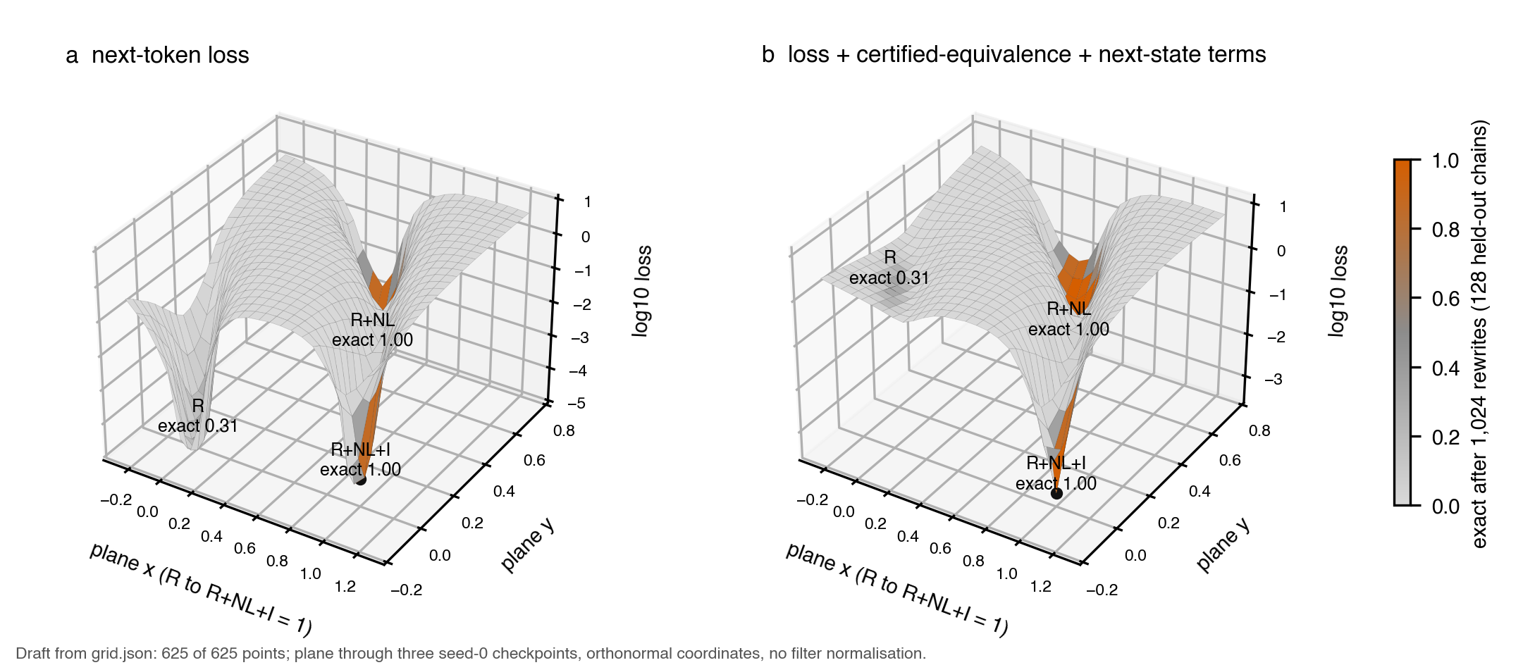
Two 3D surfaces over a plane in weight space through three trained trackers — Draft. A plane through three seed-0 checkpoints in parameter space [54]: orthonormal coordinates with the origin at R, no filter normalisation, 25 × 25 points. Height is log₁₀ of the next-token loss on 256 training chains (a), and of that loss plus the certified-equivalence and next-state terms (b). Colour is the exact final expression after 1,024 rewrites on 128 held-out chains. R has no next-state predictor, so on its side of the plane the next-state terms are read with R+NL's.

Part XI

What we learned

53Finding structure is the hard part

Our synthesis of the evidence

The project set out to give attention more than pairs. What it found is better stated in terms of combining than counting. Softmax attention compares and averages. Newton attention multiplies phases, which adds clock moves and forgets their order. Holonomy attention multiplies rotations, which keeps it. On tasks built from a group, that choice sets what a layer can learn: commuting layers stop at an exact, computable ceiling, and layers that multiply rotations go past it by learning the group's own representations, from nothing but yes/no labels.

What happens when features meet?

ComparePairwise scores
Find relevant tokens and retrieve their values.
Add phasesCommuting products
Combine clock moves. Keep content, lose order.
Compose rotationsOrdered products
Let the representation retain the order that changes the answer.

A design principle for the measured tasks. Whether it helps on natural data remains an experimental question.

Underneath that result runs a second thread, and it appears in every part of the story. The hard step was almost never representing the right structure. It was getting training to find it.

Feynman attention could represent the four-way term Match-4 needs and never found it (section 16).
Newton attention is exact precisely when it has found every character, and otherwise its accuracy grows in step with how many it has (section 20).
Softmax handed every character could, in principle, compute the answer, and stayed at chance (section 24).
The smallest faithful rotations learn A₅ fully, only more slowly; short products made long ones easier to learn (sections 29 and 32).
Two of three combined layers solved every task on one seed and failed on fresh ones (section 33).
With the loss on the answer, both models still stopped at a shortcut (section 34).
On ARC-style grids, the trained models solved none of the tasks that move the grid, while a solver that infers the operator from the examples solved all of them (section 35).

Seen this way, the language results stop looking like a separate failure. At our scale, text rewards the things that are easy to find, nearby tokens and pairwise matches, and the few gains we measured came from exactly those (a short convolution, a better local estimate). The structure our layers could represent was either rare in the data or too hard to discover, and we cannot yet tell which.

54What we would try next

Open directions

Scale the long-context result. A recurrent memory with content-driven frames beats a strengthened softmax model only once the context is long, and the frames' share grows with it (section 39). The claim worth testing is that slope: more sizes, contexts of 16,000 tokens and beyond, real kernels, and evaluations that need long-range recall. Events as the unit of memory need a router that does not drift and a way to keep exact tokens (section 40).
Infer operators from examples. Parallax-style layers fit a small linear model to the context. The ARC result suggests fitting a transformation instead: estimate the operator that maps each example input to its output, then apply it to the query. The closed-form solver shows the information is there.
Select, then compose. Real programs interleave relevant and irrelevant steps. Layers that choose which operations to compose by content, tested on longer programs against matrix recurrences and positional softmax, are the natural next experiment.
Go larger. Higher-order attention has been reported to help at billions of parameters on reasoning and code [5]. Our budget could not reach that regime.

56Methods, cost and reproducibility

How the numbers were produced

Two engines. The browser results (the SET and pointer-chase benches, and every live figure) come from this app's engine, written with jax-js [23] and run on WebGPU, so you can reproduce them in the Compare tab. The cloud results come from a JAX research harness on rented L4 and H100 GPUs.

Discipline. Puzzle results use balanced accuracy on held-out data and three seeds. Every language and later study wrote its predictions and pass/fail thresholds into the repository before its main runs, tuned each model's learning rate on its own, and matched training compute. Where a prediction was changed after a pilot, the change and the reason are recorded. Failed predictions are reported as failed.

Cost. The three language searches S0–S2 cost about $64, the S6 study $58, the group experiments about $3, the word problems about $15, the combined-layer study about $76 before we stopped it, and the dilution and ARC tests $3.76: small budgets by design, which is also why every language claim here is about small models.

Where everything is. Each study has a research note with its full protocol:

SEARCH.md: the staged language search, S0–S2
LOCAL.md: local-linear attention and Parallax, S6
FORMALISM.md: subset attention and the walk sector
GROUPS.md: groups, word problems and swap programs
THEORY.md: the theorems and exact ceilings
PRIOR_ART.md: the verified literature audit
BEYOND_REPORT.md: the combined layers
NEXT.md: loss dilution and algebraic ARC

Raw per-run results live in research/results, and every number in this article is copied from them or from these notes.

References

A. Vaswani, N. Shazeer, N. Parmar, J. Uszkoreit, L. Jones, A. N. Gomez, Ł. Kaiser, I. Polosukhin. Attention is all you need. Advances in Neural Information Processing Systems 30, 2017.
M. Hahn. Theoretical limitations of self-attention in neural sequence models. Transactions of the Association for Computational Linguistics 8, 156–171, 2020.
C. Sanford, D. Hsu, M. Telgarsky. Representational strengths and limitations of transformers. Advances in Neural Information Processing Systems 36, 2023.
J. Clift, D. Doryn, D. Murfet, J. Wallbridge. Logic and the 2-simplicial transformer. International Conference on Learning Representations, 2020.
A. Roy, T. Chou, S. S. Duvvuri, S. Chen, J. Yu, X. Wang, M. Zaheer, R. Anil. Fast and simplex: 2-simplicial attention in Triton. arXiv:2507.02754, 2025.
M. Mohsenvand. Polyformer: embracing the bitter lesson. Unpublished notebook, Complex Learning Group, 11 April, 2023.
J. Alman, Z. Song. How to capture higher-order correlations? Generalizing matrix softmax attention to Kronecker computation. International Conference on Learning Representations, 2024.
A. Kozachinskiy, F. Urrutia, H. Jimenez, T. Steifer, G. Pizarro, M. Fuentes, F. Meza, C. Buc, C. Rojas. Strassen attention: unlocking compositional abilities in transformers based on a new lower bound method. arXiv:2501.19215, 2025.
S. Chakrabarti, T. Pitassi, J. Alman. Poly-attention: a general scheme for higher order self-attention. International Conference on Learning Representations, 2026.
B. L. Davis, D. Maclagan. The card game SET. The Mathematical Intelligencer 25(3), 33–40, 2003.
F. J. Dyson. The S matrix in quantum electrodynamics. Physical Review 75, 1736, 1949.
J. Schwinger. On the Green's functions of quantized fields. I. Proceedings of the National Academy of Sciences 37, 452–455, 1951.
R. P. Feynman. Space-time approach to quantum electrodynamics. Physical Review 76, 769, 1949.
A. Chakrabarti. Lower bounds for multi-player pointer jumping. IEEE Conference on Computational Complexity, 33–45, 2007.
J. P. Ellis. TikZ-Feynman: Feynman diagrams with TikZ. arXiv:1601.05437, 2016.
E. Abbe, E. Boix-Adserà, T. Misiakiewicz. SGD learning on neural networks: leap complexity and saddle-to-saddle dynamics. COLT, 2023.
N. Nanda, L. Chan, T. Lieberum, J. Smith, J. Steinhardt. Progress measures for grokking via mechanistic interpretability. ICLR, 2023.
Y. Zuo, Y. Yin, Z. Zeng, A. Li, B. Zhu, Z. Wang. Local Linear Attention: An optimal interpolation of linear and softmax attention for test-time regression. arXiv:2510.01450, 2025.
Y. Zuo, D. Pai, Z. Zeng, A. Dewulf, S. Hu, Z. Wang. Parallax: Parameterized local linear attention for language modeling. arXiv:2605.29157, 2026.
C. Toth, P. Bonnier, H. Oberhauser. Seq2Tens: An efficient representation of sequences by low-rank tensor projections. ICLR, 2021.
H. Lou, S. Li, H. Ni. Path development network with finite-dimensional Lie group representation. Transactions on Machine Learning Research, 2024.
B. Chughtai, L. Chan, N. Nanda. A toy model of universality: reverse engineering how networks learn group operations. arXiv:2302.03025, 2023.
E. Zhang. jax-js: JAX-style arrays, autodiff and jit in the browser. Software, github.com/ekzhang/jax-js, 2025.
M. Zaheer, S. Kottur, S. Ravanbakhsh, B. Poczos, R. Salakhutdinov, A. Smola. Deep sets. NeurIPS, 2017.
M. Lezcano-Casado, D. Martínez-Rubio. Cheap orthogonal constraints in neural networks: a simple parametrization of the orthogonal and unitary group. ICML, 2019.
J. Diehl, K. Ebrahimi-Fard, N. Tapia. Time-warping invariants of multidimensional time series. Acta Applicandae Mathematicae 170:265–290, 2020.
P. Bonnier, P. Kidger, I. Perez Arribas, C. Salvi, T. Lyons. Deep signature transforms. NeurIPS, 2019.
F. Moreno-Pino, Á. Arroyo, H. Waldon, X. Dong, Á. Cartea. Rough Transformers: lightweight and continuous time series modelling through signature patching. NeurIPS, 2024.
J. Siems, T. Carstensen, A. Zela, F. Hutter, M. Pontil, R. Grazzi. DeltaProduct: improving state-tracking in linear RNNs via Householder products. NeurIPS, 2025.
B. Liu, J. T. Ash, S. Goel, A. Krishnamurthy, C. Zhang. Transformers learn shortcuts to automata. ICLR, 2023.
S. Yang, J. Kautz, A. Hatamizadeh. Gated delta networks: improving Mamba2 with delta rule. ICLR, 2025.
S. Yang et al.. PaTH attention: position encoding via accumulating Householder transformations. arXiv, 2025.
D. R. So et al.. Primer: searching for efficient transformers for language modeling. NeurIPS, 2021.
K. Jordan et al.. Muon: an optimizer for hidden layers in neural networks. blog post, 2024.
F. Chollet. On the measure of intelligence. arXiv, 2019.
J. Su, Y. Lu, S. Pan, A. Murtadha, B. Wen, Y. Liu. RoFormer: enhanced transformer with rotary position embedding. arXiv, 2021.
Z. Lin, E. Nikishin, X. O. He, A. Courville. Forgetting Transformer: softmax attention with a forget gate. ICLR, 2025.
Z. Qiu et al.. Gated attention for large language models: non-linearity, sparsity, and attention-sink-free. NeurIPS, 2025.
Z. Zhou, T. Wu, Z. Jiang, Z. Lan. Value residual learning for alleviating attention concentration in transformers. arXiv, 2024.
S. Hwang, B. Wang, A. Gu. Dynamic chunking for end-to-end hierarchical sequence modeling. ICLR, 2026.
A. Yang, D. Chiang, D. Angluin. Masked hard-attention transformers recognize exactly the star-free languages. NeurIPS, 2024.
A. Nerode. Linear automaton transformations. Proceedings of the American Mathematical Society 9, 541–544, 1958.
D. Park. Concurrency and automata on infinite sequences. Theoretical Computer Science (5th GI-Conference), LNCS 104, 167–183, 1981.
R. Milner. Communication and concurrency. Prentice Hall, 1989.
J. J. M. M. Rutten. Universal coalgebra: a theory of systems. Theoretical Computer Science 249, 3–80, 2000.
R. Givan, T. Dean, M. Greig. Equivalence notions and model minimization in Markov decision processes. Artificial Intelligence 147, 163–223, 2003.
E. van der Pol, T. Kipf, F. A. Oliehoek, M. Welling. Plannable approximations to MDP homomorphisms: equivariance under actions. AAMAS, 2020.
K. Vafa, J. Y. Chen, A. Rambachan, J. Kleinberg, S. Mullainathan. Evaluating the world model implicit in a generative model. NeurIPS, 2024.
L. de Moura, S. Ullrich. The Lean 4 theorem prover and programming language. CADE 28, LNCS 12699, 625–635, 2021.
J. Teoh, M. Tomar, K. Ahn, E. S. Hu, T. Pearce, P. Sharma, A. Krishnamurthy, R. Islam, A. Lamb, J. Langford. Next-latent prediction transformers learn compact world models. arXiv, 2025.
N. Ferns, P. Panangaden, D. Precup. Metrics for finite Markov decision processes. UAI, 2004.
A. Zhang, R. McAllister, R. Calandra, Y. Gal, S. Levine. Learning invariant representations for reinforcement learning without reconstruction. ICLR, 2021.
A. Kazemnejad, I. Padhi, K. Natesan Ramamurthy, P. Das, S. Reddy. The impact of positional encoding on length generalization in transformers. NeurIPS, 2023.
H. Li, Z. Xu, G. Taylor, C. Studer, T. Goldstein. Visualizing the loss landscape of neural nets. NeurIPS, 2018.
N. Lee, Z. Cai, A. Schwarzschild, K. Lee, D. Papailiopoulos. Self-improving transformers overcome easy-to-hard and length generalization challenges. ICML, 2025.
B. Hui, J. Yang, Z. Cui et al.. Qwen2.5-Coder technical report. arXiv, 2024.
M. Nye, A. J. Andreassen, G. Gur-Ari, H. Michalewski, J. Austin, D. Bieber, D. Dohan, A. Lewkowycz, M. Bosma, D. Luan, C. Sutton, A. Odena. Show your work: scratchpads for intermediate computation with language models. arXiv, 2021.

1What this is about

The short version

2The puzzles

3How a puzzle becomes tokens

4Attention compares pairs

5Why pairs are blind to SET

6Scoring whole triples

7Cheaper relatives, and what they miss

8A head built by hand

9What training shows

10Four cards need a four-way term

SET: three cards sum to 0

Four cards sum to 0

11Where Feynman diagrams come from

12Summing all the diagrams at once

13Feynman attention

14Making it train

15What Feynman attention learns

16Big relations do not grow from small ones

17A group is a rule for combining

18Relations as agreeing phases

19Newton's shortcut

20Newton attention

21Small relations teach large ones

22What we tried on text

23What the language result means

24Good coordinates are not enough

25When order changes the answer

26Operations as rotations

27Holonomy attention

28The price of forgetting order

A₄ · tetrahedral rotations

A₅ · icosahedral rotations

29The heads learn the group

30What is proved

31Running small programs

32Long products: word problems

33One layer with everything

34Is the loss hiding it?

35Grid puzzles in the style of ARC

36Two memories on text

37The models find events on their own

38A stronger baseline erases it at short range

39What pays at long context

40Events as the unit of memory

41Why text rewards resets, not groups

42Why training lands near exact

43One state for equivalent histories

44Lean as the referee

45What is shown, and what is not

46Harder tests of the same result

47The three clauses in one loss

48What the exact state is, and what it saves

49Natural proofs: the kind of step, not the terms

50Reading out verdicts, not strings

51Latent execution without chain of thought

Where the step is arithmetic

5224 October 2026: what the review round established

The attribution factorial (24 October 2026)

Two controls (24 October 2026)

Soft checkers (24 October 2026)

Three ingredients of exactness at length (24 October 2026)

An idea, not a result: Nerode self-distillation (24 October 2026)

A cut through weight space (24 October 2026, draft)

53Finding structure is the hard part

54What we would try next

55What is new here, and what is not

56Methods, cost and reproducibility